How to Find Duplicates in Excel?

Are you struggling to manage large Excel datasets and spot duplicate entries? You're not alone! Many users face the challenge of handling duplicate data that sneaks into spreadsheets, leading to errors and disrupting analysis. But don't worry - there are multiple ways to effectively tackle this problem, and knowing How to Find Duplicates in Excel can be a game-changer for data accuracy.

In this blog, we’ll show you step-by-step methods that will turn this tricky task into a seamless process. By mastering How to Find Duplicates in Excel, you can ensure that your data remains tidy, accurate, and ready for action. Ready to clean up your spreadsheets? Let's dive in!

Table of Contents

1) What are Duplicates in Excel?

2) Five Methods to Identify Duplicates in Excel

a) Conditional Formatting

b) Conditional Formatting (Specific Occurrence)

c) Using Formulas (Custom Rules)

d) COUNTIF Formula

e) Pivot Table

3) Methods to Remove Duplicates in Excel

4) How to Find Duplicate Rows in Excel?

5) Conclusion
 

 

What are Duplicates in Excel?

In Excel, duplicates are repeated or identical values that appear more than once within a dataset. These can occur in a single column or across multiple columns. Identifying and managing duplicates is crucial to ensure data accuracy and reliability, preventing errors in analysis and reporting. Duplicates might include repeated entries of customer names, product codes, or identical transaction records.

 

Five Methods to Identify Duplicates in Excel

Now that you know what Duplicates are, let’s have a look at How to Find Duplicates in Excel. Here's a closer look:

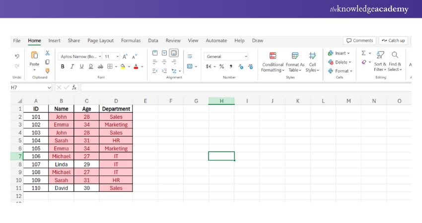
Method 1: Conditional Formatting 

Step 1. Select the range of cells where you want to identify duplicates.

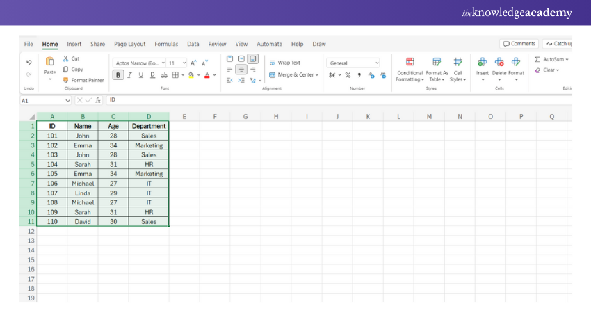
Step 2. Go to the Home tab in Excel.

Step 3. Click on Conditional Formatting in the ribbon.

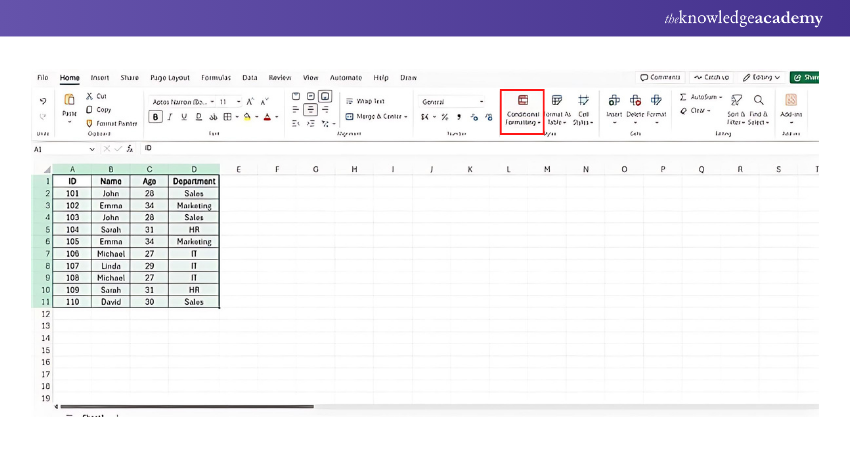
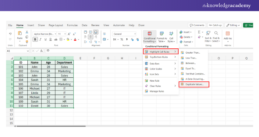
Step 4. Choose Highlight Cells Rules and then select Duplicate Values.

Step 5. In the popup, choose how you want to format the duplicate cells (e.g., with a colour).

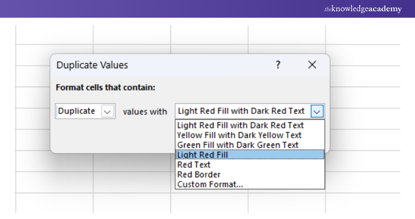
Step 6. Click OK, and Excel will highlight all the duplicate values in the selected range.

Method 2: Conditional Formatting (Specific Occurrence) 

Step 1. Select the range of cells where you want to check for specific occurrences of duplicates.

Step 2. Go to the Home tab.

Step 3. Select Conditional Formatting and then choose New Rule.

Step 4. In the popup, select Use a formula to determine which cells to format.

Step 5. Enter a formula, like =COUNTIF($A$1:$A$100,A1)=2 to highlight cells that appear exactly twice.

Step 6. Choose your desired formatting (colour), and click OK. Excel will highlight values that meet the specific criteria.

Enhance your Excel skills by learning Microsoft Excel VBA and Macro Training. Automate tasks and improve productivity now!

Method 3: Using Formulas (Custom Rules with IF)

Step 1. In a new column (e.g., E2), enter the following formula:

=IF(COUNTIF(B$2:B$11, B2)>1, "Duplicate", "Unique")

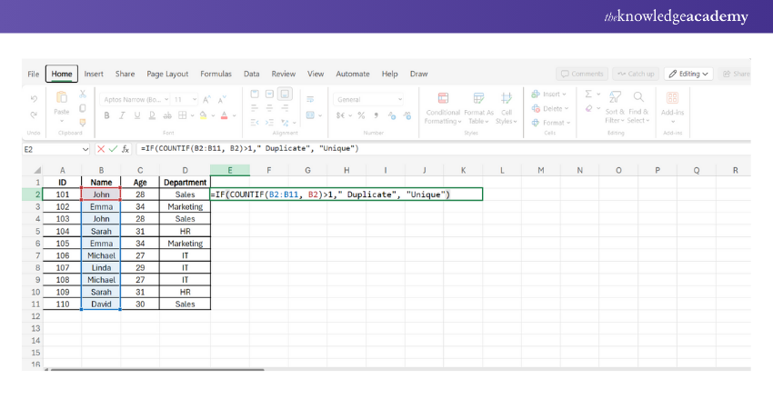
Step 2. Drag the formula down across the range to apply it to all rows.

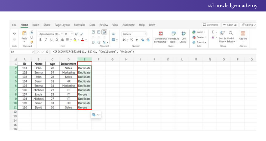
Step 3. Duplicates will be flagged based on the conditions defined in the formula.

Method 4: COUNTIF Formula

Step 1. In a new column (e.g., F2), enter the following formula:

=COUNTIF(B$2:B$11, B2)

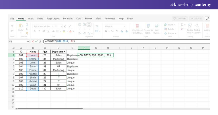
Step 2. Drag the formula down across the range to apply it to all rows.

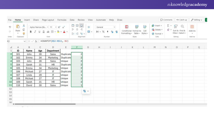
Step 3. This formula will count how many times each name appears in the Name column. Any value greater than 1 indicates a duplicate.

Method 5: Pivot Table

Step 1. Select the range A1.

Step 2. Go to Insert > PivotTable and choose where to place the Pivot Table (new or existing worksheet).

Step 3. In the PivotTable Field List, drag the Name field to the Rows section.

Step 4. Drag the Name field to the Values section (this will show the count of each name).

Step 5. The Pivot Table will now display each name and how many times it appears. Names with a count greater than 1 are duplicates.

Want to learn more about organising data? Discover How to Create Pivot Table in Excel and improve your Excel skills to the next level. 

Methods to Remove Duplicates in Excel

Here are the different methods to remove duplicates in Excel, each providing a specific way to clean your data by eliminating repeated entries:

Method 1: Remove Duplicates Tool (Quick and Easy)

Step 1. Select your data range. If you want to remove duplicates from the entire dataset, select all relevant columns (e.g., A1).

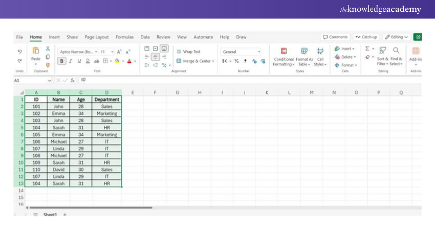
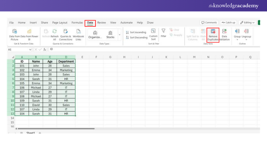
Step 2. Go to the Data tab.

Step 3. Choose Remove Duplicates in the Data Tools group.

Step 4. In the dialogue box, select the columns you want Excel to check for duplicates. If you want to remove duplicates based on the entire row, make sure all columns are checked.

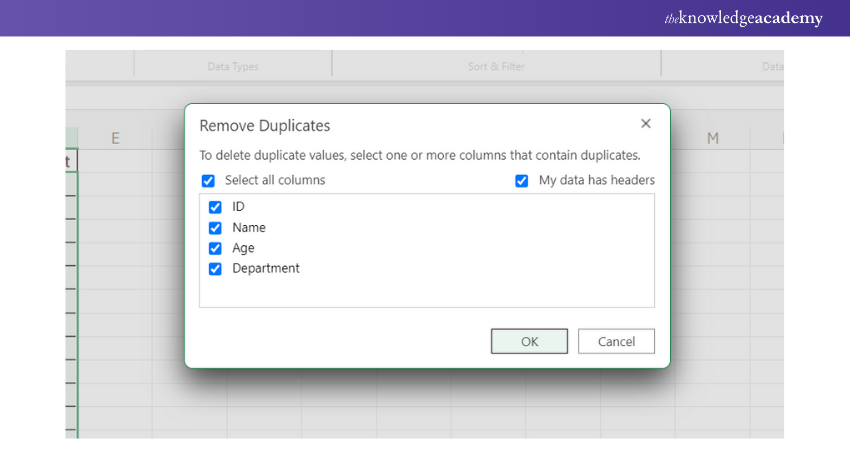
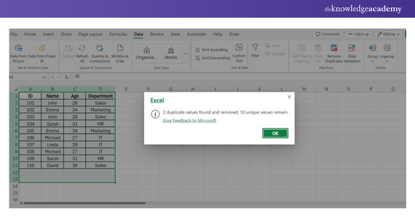
Step 5. Click OK. Excel will remove any duplicate rows, keeping only the first occurrence.

Method 2: Advanced Filter 

Step 1. Select your data range, including headers (e.g., A1).

Step 2. Go to the Data tab.

Step 3. Click Advanced in the Sort & Filter group.

Step 4. In the Advanced Filter dialogue box:

a) Choose Copy to another location.

b) In the List range, ensure your dataset is selected (e.g., A1).

c) In the Copy to field, select where you want to paste the unique records (e.g., F1).

d) Check the Unique records only box.

Step 5. Click OK. Excel will paste only the unique rows to the new location.

Method 3: Pivot Table (For Identifying and Manually Removing Duplicates)

Step 1. Select your data range (e.g., A1).

Step 2. Go to Insert > PivotTable.

Step 3. In the PivotTable Field List, drag each column (ID, Name, Age, Department) to the Rows section.

Step 4. Drag any column (e.g., ID) to the Values section and set it to Count.

Step 5. Any row with a count greater than 1 is a duplicate.

Step 6. Manually go back to the original dataset and remove the duplicates.

Advance your business insights – sign up for the Business Analytics With Excel Course and become an analytics expert!

How to Find Duplicate Rows in Excel?

Let’s explore simple yet effective methods to help you find and manage duplicate rows in Excel.

Method 1: Conditional Formatting to Highlight Duplicate Rows

Step 1. Select your data range (including all relevant columns, e.g., A1).

Step 2. Go to the Home tab.

Step 3. Click on Conditional Formatting > New Rule.

Step 4. In the dialogue box, select Use a formula to determine which cells to format.

Step 5. Enter the following formula to check for duplicate rows (assuming your data starts from row 2):

=COUNTIFS($A$2:$A$11, $A2, $B$2:$B$11, $B2, $C$2:$C$11, $C2, $D$2:$D$11, $D2)>1

Step 6. Click Format, choose your preferred formatting (e.g., a highlight colour), and click OK.

Step 7. Click OK again to apply the rule. Excel will now highlight the duplicate rows.

Method 2: Remove Duplicates Tool

Step 1. Select your data range (e.g., A1).

Step 2. Go to the Data tab.

Step 3. Click on Remove Duplicates.

Step 4. In the dialogue box, check all columns to ensure Excel checks the entire row for duplicates.

Step 5. Click OK. Excel will remove any duplicate rows and provide a summary of how many duplicates were found and removed.

Enhance your Excel skills to new heights with our expert-led Microsoft Excel Course - register now and start excelling!

Conclusion 

Mastering How to Find Duplicates in Excel is essential for maintaining clean, accurate data. By using methods like Conditional Formatting, COUNTIF, and Pivot Tables, you can efficiently identify and manage duplicates. Say goodbye to data errors and embrace a cleaner, more efficient spreadsheet experience!

Transform your accounting workflow with our Excel for Accounting Course - sign up now!