We may not have the course you’re looking for. If you enquire or give us a call on + 1-866 272 8822 and speak to our training experts, we may still be able to help with your training requirements.
Training Outcomes Within Your Budget!
We ensure quality, budget-alignment, and timely delivery by our expert instructors.

Struggling to keep track of important data while scrolling through large Excel sheets? Learning How to Freeze Panes in Excel is a simple yet powerful feature that locks specific rows or columns in place. This makes it easier to manage and analyse data without losing sight of key information.
Imagine effortlessly navigating your spreadsheets with crucial headers and data always in view. Freezing panes can transform your data management experience, making your work smoother and more efficient.
Ready to enhance your Excel skills? This blog helps you discover How to Freeze Panes in Excel and unlock a more organised and productive workflow.
Table of Contents
1) Understanding Freeze Panes
2) How Do Freeze Panes Work?
3) Other Viewing Options
4) Benefits of Using Freeze Panes
5) Impact of Freeze Panes on Sorting and Filtering Data
6) Difference Between Frozen Rows and Locked Rows
7) Conclusion
Understanding Freeze Panes
Freeze Panes is a feature in Excel that helps you lock certain rows or columns. But they remain visible as you scroll through the rest of the worksheet. This is especially useful when working with large datasets, as it ensures that headers or key information remain visible. By freezing panes, you can easily reference specific data points without losing track of your position in the spreadsheet.
How Do Freeze Panes Work?
Freeze Panes eliminates visual barrier that keeps the selected rows or columns from moving when you scroll. This feature can be applied to the top row, the first column, or any selected section of the sheet. Let's examine the different ways you can use Freeze Panes in Excel.
1) Freezing the Top Row
Freezing the top row is a common use of this feature, especially when the top row contains headers or labels for your data. To freeze the top row, go through these steps:
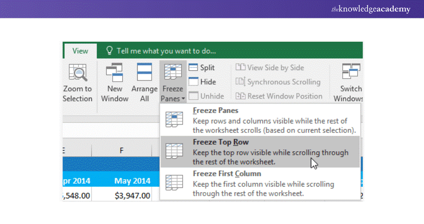
1) Go to the View tab on the Excel ribbon.
2) Click on the Freeze Panes dropdown menu.
3) Select "Freeze Top Row."
Once you have frozen the top row, it will remain visible as you scroll down through the rest of the data. This is particularly useful for keeping headers in view when working with large tables.
2) Unfreezing Panes
If you need to unfreeze the panes at any point, the process is straightforward:
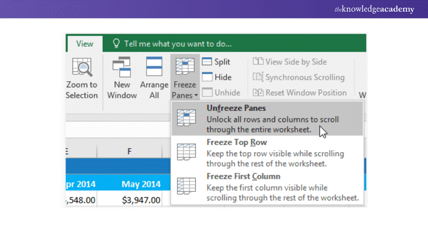
1) Go back to the View tab on the Excel ribbon.
2) Click on the Freeze Panes dropdown menu.
3) Select "Unfreeze Panes."
This action will remove any frozen rows or columns, allowing the entire sheet to scroll freely.
Learn to create Gantt Charts in Excel with our Excel Training with Gantt Charts- Sign up now!
3) Freezing Rows
In addition to the top row, you can freeze multiple rows in your worksheet. To do this:
1) Click on the row below the row(s) you want to freeze. For example, if you want to freeze rows 1 and 2, click on row 3.
2) Go to the View tab.
3) Click on the Freeze Panes dropdown menu.
4) Select "Freeze Panes."
This will keep the selected rows visible as you scroll through the rest of the sheet.
4) Freezing Columns
Similarly, you can freeze columns to keep them visible while scrolling horizontally. Here's how:
1) Click on the column to the right of the column(s) you want to freeze. For example, to freeze columns A and B, click on column C.
2) Go to the View tab.
3) Click on the Freeze Panes dropdown menu.
4) Select "Freeze Panes."
Now, the selected columns will stay visible as you scroll to the right.
Other Viewing Options
Excel offers several other viewing options that can enhance your data navigation experience.
1) Opening a New Window
If you want to view different parts of the same worksheet simultaneously, you can open a new window:
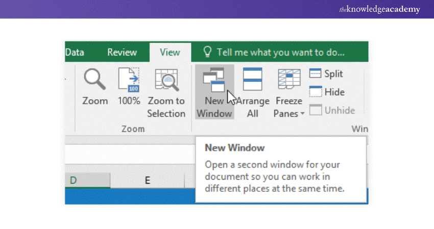
1) Go to the View tab.
2) Click on "New Window."
This opens a new window for the current workbook, allowing you to view and work on different sections at the same time.
2) Splitting Panes
Splitting panes is another useful feature for viewing different sections of your worksheet:
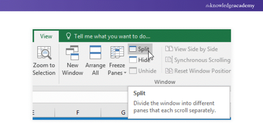
1) Click on the cell where you want to split the window.
2) Go to the View tab.
3) Click on "Split."
This will create a horizontal and vertical split, allowing you to scroll different sections independently.
3) Using the Magic Freeze Button
The Magic Freeze Button is a feature that automatically freezes rows and columns based on the selected cell. To use it:
1) Select the cell below and to the right of the rows and columns you wish to freeze.
2) Go to the View tab.
3) Click on the Freeze Panes dropdown menu.
4) Select "Magic Freeze Button."
This will freeze all rows above and columns to the left of the selected cell.
Benefits of Using Freeze Panes
Freezing panes can transform users' data management experience. Let’s discuss some of the benefits of using Freeze Panes here:
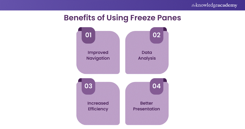
1) Improved Navigation: Keep headers and important information in view while scrolling.
2) Data Analysis: Easily compare different parts of your dataset without losing track of your position.
3) Increased Efficiency: Save time by not having to scroll back and forth to reference specific data points.
4) Better Presentation: Enhance the readability and presentation of your data, especially when sharing with others.
Gain in-depth knowledge of VBA with our Microsoft Excel VBA and Macro Training- register now!
Impact of Freeze Panes on Sorting and Filtering Data
Freeze Panes do not affect Excel's sorting and filtering capabilities. You can still sort and filter data as usual, and the frozen rows or columns will remain in place. This is particularly helpful when working with large datasets where maintaining the visibility of key information is crucial.
Difference Between Frozen Rows and Locked Rows
1) Functionality:
Frozen Rows: Focus on visibility and ease of navigation.
Locked Rows: Focus on security and data protection.
2) Effect on User Interaction:
Frozen Rows: Allow scrolling while keeping specific rows in view.
Locked Rows: Prevent editing but do not impact scrolling.
3) Common Use Cases:
Frozen Rows: Keeping header rows visible for large datasets.
Locked Rows: Protecting critical data in collaborative environments.
Understanding these differences helps in effectively managing and protecting data in spreadsheets, ensuring both ease of use and data integrity.
Conclusion
Freeze Panes is a flexible and robust function in Excel that improves your capacity to move, examine, and display extensive datasets. Understanding How to Freeze Panes in Excel can greatly enhance your workflow and productivity. It keeps headers visible or concentrates on specific data poinpoints. Discover these functionalities to improve the efficiency and streamline of your data management responsibilities.
Understand how to collaborate and share in Excel with our Microsoft Excel Course today!
Frequently Asked Questions

The Freeze Panes rule in Excel refers to the ability to freeze specific rows or columns in place. But they remain visible while you scroll through your worksheet. This feature helps keep important information, such as headers or key data points, in view as you navigate large datasets. This is how you can use the Freeze Pane's rule.

When you use the Freeze Panes option on specific rows, those rows become locked in place and remain shown as you scroll down the sheet. The rest of the rows below the frozen section will scroll normally, allowing you to navigate the data without losing sight of the important information in the frozen rows.

To remove Freeze Panes in Excel, go to the View tab on the ribbon in Excel, click on the Freeze Panes dropdown menu, and select "Unfreeze Panes." This will remove any frozen rows or columns, allowing the entire sheet to scroll freely. Make your work efficient and organised with Freeze Panes.

The Knowledge Academy takes global learning to new heights, offering over 30,000 online courses across 490+ locations in 220 countries. This expansive reach ensures accessibility and convenience for learners worldwide.
Alongside our diverse Online Course Catalogue, encompassing 17 major categories, we go the extra mile by providing a plethora of free educational Online Resources like News updates, Blogs, videos, webinars, and interview questions. Tailoring learning experiences further, professionals can maximise value with customisable Course Bundles of TKA.

The Knowledge Academy’s Knowledge Pass, a prepaid voucher, adds another layer of flexibility, allowing course bookings over a 12-month period. Join us on a journey where education knows no bounds.

The Knowledge Academy offers various Microsoft Excel Courses, including the Microsoft Excel Course, Microsoft Excel VBA And Macro Training, and Excel For Accounting Course. These courses cater to different skill levels and provide comprehensive insights into How to Use Excel.
Our Office Applications Blogs cover a range of topics related to Office Applications, offering valuable resources, best practices, and industry insights. Whether you are a beginner or looking to advance your Office Applications Skills, The Knowledge Academy's diverse courses and informative blogs have got you covered.
Upcoming Office Applications Resources Batches & Dates
Date
 Microsoft Excel Course
Fri 10th Jan 2025
Fri 14th Feb 2025
Fri 11th Apr 2025
Fri 23rd May 2025
Fri 8th Aug 2025
Fri 26th Sep 2025
Fri 21st Nov 2025


 Top Rated Course


 If you wish to make any changes to your course, please


