We may not have the course you’re looking for. If you enquire or give us a call on +357 26030221 and speak to our training experts, we may still be able to help with your training requirements.
Training Outcomes Within Your Budget!
We ensure quality, budget-alignment, and timely delivery by our expert instructors.

Imagine taking just a few clicks to turn a mountain of raw data into a clear, insightful summary—that's the power Pivot Tables in Excel offer! These versatile tools transform chaotic spreadsheets into easy-to-read reports that spotlight exciting patterns, trends and key takeaways, helping you make data-driven decisions with confidence. This blog explores How to Create a Pivot Table in Excel, detailing every step and the essentials to help you become a data pro. So, read on and transform your Data Analysis game!
Table of Contents
1) What is a Pivot Table in Excel?
2) What is the Use of Pivot Table in Excel?
3) How to Create a Pivot Table in Excel? Six Easy Steps
a) Step 1: Fill out a Set of Rows and Columns With Your Data
b) Step 2: To Make Your Pivot Table, Mark the Cells
c) Step 3: Sort Your Data by a Specific Property
d) Step 4: Add a Field by Dragging it Into the "Row Labels" Section
e) Step 5: Add a Field by Dragging it Into the “Values Area”
f) Step 6: Adjust Your Calculations as Needed
4) Pivot Table Essentials
5) Conclusion
What is a Pivot Table in Excel?
A Pivot Table is a statistics tool that summarises and reorganises selected rows and columns of data in a database table or spreadsheet to obtain a desired report. The tool does not change the database or spreadsheet itself; it simply “pivots” the data to view it from different perspectives.
Pivot Tables can be handy when large amounts of data are too time-consuming to calculate by hand. A Pivot Table can identify sums, averages, ranges, or outliers, among other data processing functions.
What is the Use of Pivot Table in Excel?
A Pivot Table enables users to answer business questions with minimal effort. Some of the common uses of Pivot Tables include:
1) To calculate sums or averages in business situations. For instance, counting sales by region or department.
2) To showcase totals as a percentage of a whole. For example, comparing sales of a specific product to total sales.
3) To generate a list of unique values. For instance, showing which states or countries a product order has come from.
4) To create a 2x2 table summary of a complex report.
5) To identify the maximum and minimum values in a dataset.
How to Create a Pivot Table in Excel? Six Easy Steps
Now that the basic idea behind Pivot Tables has been covered, it’s time to dive into the process of creating one. The following six steps will help simplify the entire path towards creating an effective Pivot Table that will help you summarise vital and complex datasets in no time
Step 1: Fill out a Set of Rows and Columns With Your Data
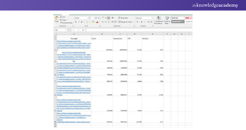
Every Pivot Table in basic Excel begins with a fundamental Excel table containing all your data. Enter your values into the designated rows and columns to build the table. Use the top row or column to group your values according to what they stand for.
For example, if you want to create a table that records the blog post-performance data, you should have five columns that bring out the categorised data. Follow the steps below to understand the process.
Step 2: To Make Your Pivot Table, Mark the Cells
After entering the data in your Excel spreadsheet, mark the cells you want to compile in a Pivot Table. Click on “Insert” and then select the “Pivot Table” icon. To make a Pivot Table, highlight the cells you want to use.
You may choose whether to launch this Pivot Table in a new worksheet or keep it in the current worksheet. Additionally, it will specify your cell range in the choice box. At the bottom of your Excel worksheet, you can navigate any newly opened sheets. After selection, click OK.
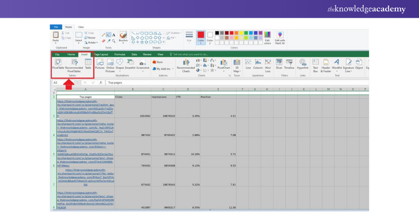
Note: If you are using the latest version of MS Excel, then the tables option under the “Insert” option, you will find a separate section of tables. Then, click on the “Tables” icon to select Pivot Table.
Master Accounting skills using Microsoft Excel in our comprehensive Excel for Accounting Course – Sign up now!
Step 3: Sort Your Data by a Specific Property
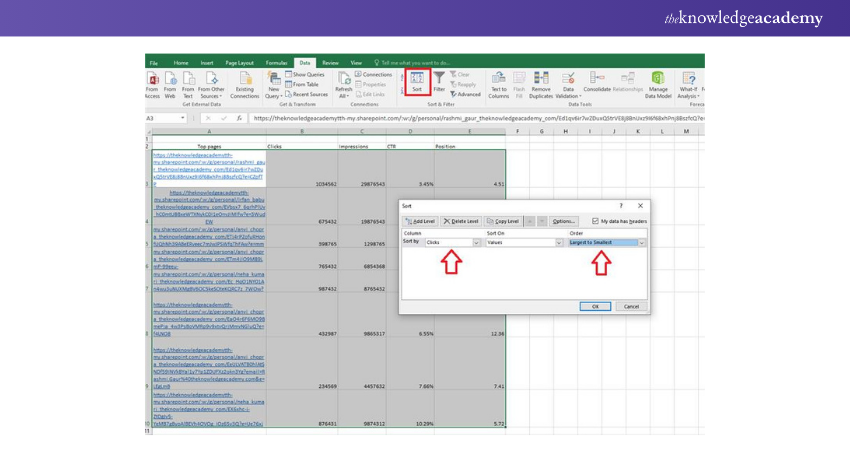
After creating the Pivot Table, right-click the values to be sorted in the data and select the sorting order you desire to use. This order can be ascending or descending in nature and is generally used for checking on a specific property within the Pivot Table.
Step 4: Add a Field by Dragging it Into the "Row Labels" Section
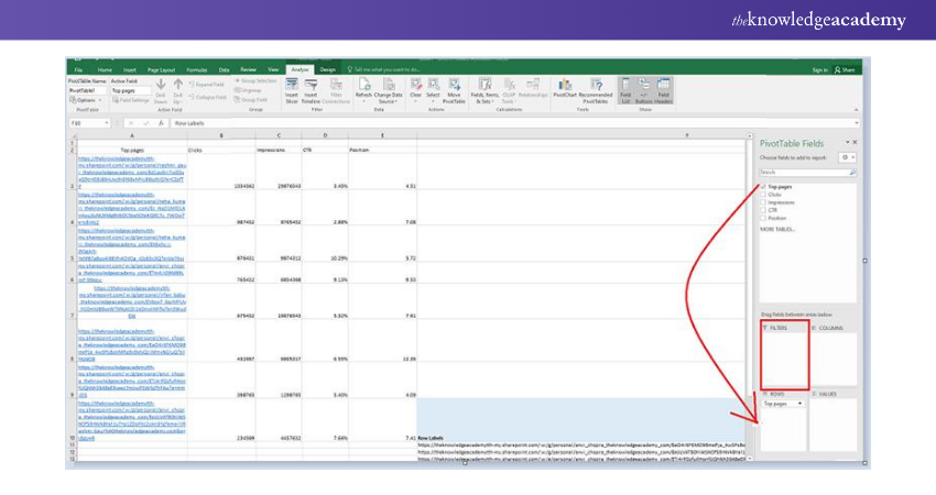
When Step 2 is finished, Excel will produce a blank Pivot Table for you. The next step is to drag and drop a field into the Row Labels section with a label that matches the names of the columns in your spreadsheet. By doing so, you can choose the specific identifier—blog post title, product name, etc.—by which the Pivot Table will arrange your data.
To organise blog data by post title, you must click and drag the “Top pages” field to the “Row Labels” area.
Step 5: Add a Field by Dragging it Into the “Values Area”
The next step is to add some values by dragging a field into the Values box once you have decided how to organise your data.
Let's use the blogging data example again. So, if you want to sum up views of blog posts by title, drag the "Views" field into the Values box to achieve this.
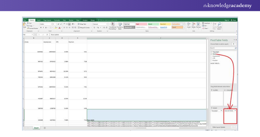
Step 6: Adjust Your Calculations as Needed
According to what you want to calculate, you can easily modify the default calculation to anything else, such as average, maximum, or minimum.
Finally, you can adjust your calculations as per your requirements. Follow the steps in the succeeding images:
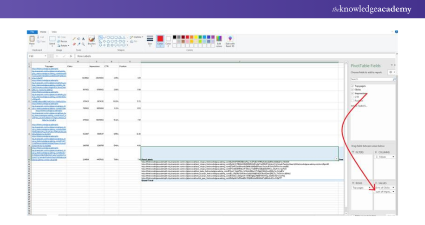
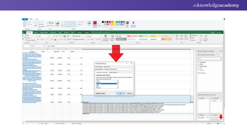
To access the menu, click on the tiny upside-down triangle next to your value and choose Value Field Settings. Follow the image below:
Master the essential functions of Excel in Business Analytics in our up-to-date Business Analytics With Excel Course – Register now!
Drag and drop the fields into the value box and then to the filter box to find the actual position of the rows and columns. Follow the image below:
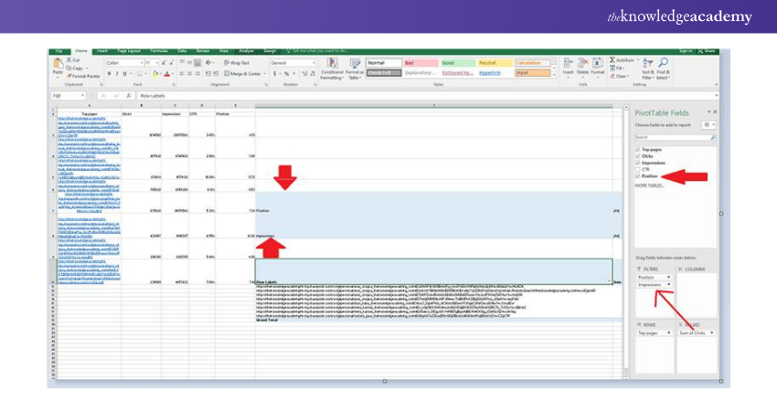
Now, you can find the total of the sum of clicks, the sum of Click Through Rate (CTR), along with the position and impressions of the blog post. Follow the image below:
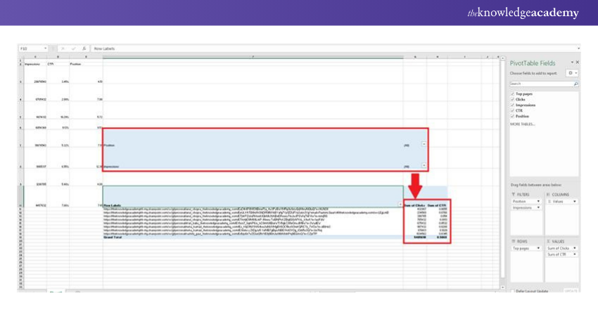
Finally, when you have categorised your data as per your requirement, save your work and use it as and when needed. The above steps will give you a clear idea of How to Create A Pivot Table in Excel.
Build your career as a Data Analyst. Check out our Data Analysis Training Using MS Excel Course today!
Pivot Table Essentials
Some tasks are unavoidable when creating and using Pivot Tables. These step-by-step instructions are essential will assist you with these tasks and explore the full potential of Pivot Tables

How to Create a Pivot Table With Multiple Columns
These steps will help you create a multi-columned Pivot Table:
a) Select Data: Select the data you want to include in your Pivot Table, including column headers.
b) Insert Pivot Table: Go to the "Insert" tab in the Excel ribbon and click on the “PivotTable” button.
c) Choose Data Range: In the “Create PivotTable” dialog box, ensure the correct range is automatically selected, and choose where you want to place the Pivot Table, such as a new or existing worksheet.
d) Designate Multiple Columns: In the PivotTable "Field List", drag and drop the fields to be included as column labels to the “Columns” area. These fields will be displayed as multiple columns in the Pivot Table.
e) Add Row Labels and Values: Drag and drop the fields you want to summarise or display as row labels to the “Rows” area.
How to Copy a Pivot Table?
These are the steps to follow if you want to copy a Pivot Table:
a) Select Entire Pivot Table: Click anywhere within the table to see selection handles around the table.
b) Copy the Table: Right-click and select “Copy” from the context menu, or use Ctrl+C on the keyboard.
c) Choose the Destination: Go to the location on the worksheet where the copied Pivot Table must be pasted.
d) To Paste the Pivot Table, Right-click on the destination cell and pick “Paste” from the context menu or use Ctrl+V on the keyboard.
e) Adjust the Pivot Table Range: In case the copied table overlaps with existing data, you must adjust the range. Click and drag the pasted Pivot Table's corner handles to resize it.
How to Sort a Pivot Table?
These two simple steps can sort any Pivot Table:
a) Go to PivotTable tab: Once the Pivot Table is selected, go to the “PivotTable Analyse” or “PivotTable Tools” tab on the Excel ribbon.
b) Sort Pivot Table: In the “Sort” group, click on the “Sort Descending” button (Z to A) or “Sort Ascending” button (A to Z).
How to Delete a Pivot Table?
To delete a Pivot Table in Excel, follow these steps:
a) Select Pivot Table: Click anywhere within the Pivot Table.
b) Delete the Pivot Table: Consider these three options:
a) Press the “Backspace” or “Delete” key on the keyboard.
b) Right-click on the Pivot Table and choose “Delete” from the context menu.
c) Go to the “PivotTable Tools” or “PivotTable Analyze” tab on the Excel ribbon, click on the “Options” or “Design” button, and select “Delete” from the dropdown menu.
How to Group Dates in Pivot Tables?
Follow these steps to group dates in a Pivot Table in Excel:
a) Ensure That Date Column is in Proper Date Format: If not, format the column as a date.
b) Select Cell: Pick a cell within the date column in the Pivot Table.
c) Choosing “Group”: Right-click and select “Group” from the context menu.
d) Grouping Option: When the Grouping dialog box appears, choose the grouping option that fits your needs, such as days, months, quarters, or years. You can select multiple options by holding down the Ctrl key while making selections.
e) Adjust Dates: Adjust the start and end dates if needed and click “OK” to apply the grouping.
How to Add a Calculated Field in a Pivot Table?
Follow these steps if you are trying to add a calculated field in a Pivot Table in Excel:
a) Select Cell: Select any cell within the Pivot Table and go to the Excel ribbon's “PivotTable Analyse” or “PivotTable Tools”.
b) Go to “Calculations” Group: In the “Calculations” group, click on the “Fields, Items & Sets” button and pick “Calculated Field” from the dropdown menu.
c) Enter a Name: Once the “Insert Calculated Field” dialog box appears, enter a name for the calculated field in the “Name” field.
d) Enter Formula: Insert the formula for the calculated field in the “Formula” field. You can use mathematical operators (+, -, *, /) and references to other fields.
e) Click “OK”: Finally, click OK to add the calculated field to the table.
How to Remove Grand Total From a Pivot Table?
These steps will help you remove the grand total from a Pivot Table:
a) Select Cell: Click on any cell within the Pivot Table and navigate to the “PivotTable Analyse” or “PivotTable Tools” tab.
b) Open Field Settings: Click on the “Field Settings” button in the “PivotTable Options” group.
c) Access Dialog Box: The “PivotTable Field Settings” or “PivotTable Options” dialog box will appear.
d) Excel Version-specific Steps:
a) For Excel 2013 and earlier versions: Go to the “Subtotals & Filters” tab and uncheck the box next to “Grand Total.”
b) For Excel 2016 and later versions: Navigate to the “Totals & Filters” tab and uncheck the box next to “Show grand totals for rows/columns.”
e) Click “OK” to apply the changes.
Conclusion
In conclusion, learning How to Create a Pivot Table in Excel can be a game-changer for anyone dealing with data. This simple yet powerful tool lets you summarise and analyse information effortlessly, transforming complex datasets into actionable insights. With practice, you can streamline your workflow, gain deeper data insight, and make better data-driven decisions.
To learn in detail to create advanced formulas, macros, and much more, you can sign up for our Microsoft Excel Expert MO201 Course now!
Frequently Asked Questions

Excel functions such as VLOOKUP, SUMIFS, COUNTIFS, and AVERAGEIFS complement the use of Pivot Tables for more advanced analyses. These functions allow users to perform specific calculations and retrieve data from large datasets, enhancing the capabilities of Pivot Tables.

To maintain accuracy in a Pivot Table over time, users can regularly update the data source by refreshing the Pivot Table. They can also automate data updates using features like Power Query or Excel Tables, ensuring that the Pivot Table reflects the most current data.

The Knowledge Academy takes global learning to new heights, offering over 30,000 online courses across 490+ locations in 220 countries. This expansive reach ensures accessibility and convenience for learners worldwide.
Alongside our diverse Online Course Catalogue, encompassing 17 major categories, we go the extra mile by providing a plethora of free educational Online Resources like News updates, Blogs, videos, webinars, and interview questions. Tailoring learning experiences further, professionals can maximise value with customisable Course Bundles of TKA.

The Knowledge Academy’s Knowledge Pass, a prepaid voucher, adds another layer of flexibility, allowing course bookings over a 12-month period. Join us on a journey where education knows no bounds.

The Knowledge Academy offers various Microsoft Excel Courses, including Microsoft Excel Course, Business Analytics with Excel and Excel Training with Gantt Charts. These courses cater to different skill levels, providing comprehensive insights into How to Create a Project Plan in Excel.
Our Office Applications Blogs cover a range of topics related to Microsoft Excel, offering valuable resources, best practices, and industry insights. Whether you are a beginner or looking to advance your Excel skills, The Knowledge Academy's diverse courses and informative blogs have you covered.
Upcoming Office Applications Resources Batches & Dates
Date
 Microsoft Excel Course
Mon 13th Jan 2025
Mon 10th Mar 2025
Mon 7th Apr 2025
Mon 9th Jun 2025
Mon 8th Sep 2025
Mon 1st Dec 2025


 Top Rated Course


 If you wish to make any changes to your course, please


