How to Use Conditional Formatting in Excel?

Envision your data could speak to you, highlighting the most important numbers without you lifting a finger. Sounds magical, right? That’s exactly what Conditional Formatting does! It’s like turning your plain spreadsheet into a vibrant canvas, where key figures glow, trends reveal themselves, and outliers jump off the page. Whether you're tracking sales, performance, or data, knowing How to Use Conditional Formatting in Excel is your secret weapon for making key information stand out.

In this blog, we’ll walk you through How to Use Conditional Formatting in Excel, from creating new rules to applying them to your data. You’ll learn how to highlight data, apply multiple rules, and even use preset styles for visual flair. Ready to unlock Excel’s formatting power? Let’s dive in!

Table of Contents

1) What is Conditional Formatting in Excel?

2) How to Use Conditional Formatting in Excel

3) Types of Conditional Formatting Rules and Styles

4) How to Copy Excel Conditional Formatting?

5) How to Clear Conditional Formatting Rules?

6) Conclusion

What is Conditional Formatting in Excel?

Conditional Formatting in Excel is a powerful feature that applies custom formatting to cells based on specific criteria, helping to visually emphasise important data. It highlights patterns, trends, or exceptions, making it easier to analyse and interpret large datasets.

Key uses of Conditional Formatting include:

a) Differentiating values, such as highlighting cells above or below a certain threshold.

b) Applying color scales, data bars, or icon sets for visual comparison.

c) Automatically flagging data that meets specific conditions (e.g., duplicates or top/bottom performers).

d) Transforming raw data into visually appealing insights for better decision-making.
 

 
 

How to Use Conditional Formatting in Excel?

The following are the steps to create a new Conditional Formatting rule in Excel, allowing you to highlight key data based on custom criteria, making your analysis more effective and visually appealing.

1) Creating a New Conditional Formatting Rule

To add a new Conditional Formatting rule in Excel, follow these steps:

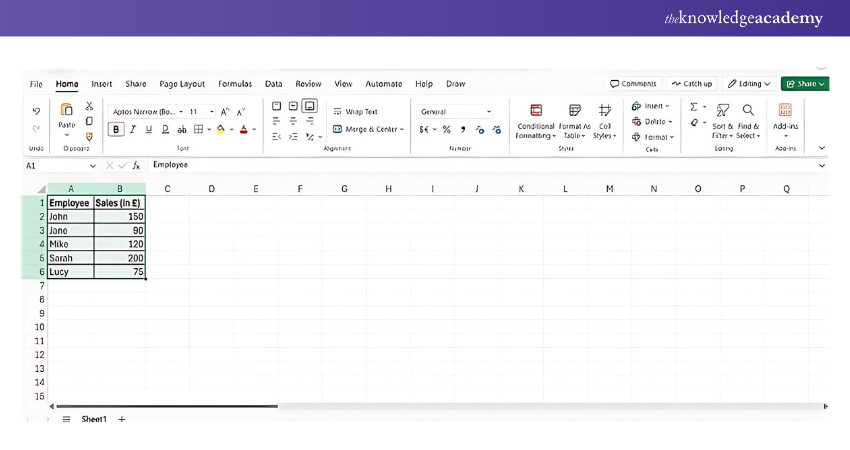
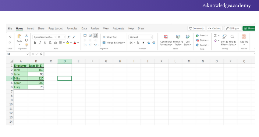
Step 1. Choose the range of cells where do you would like to apply the rule.

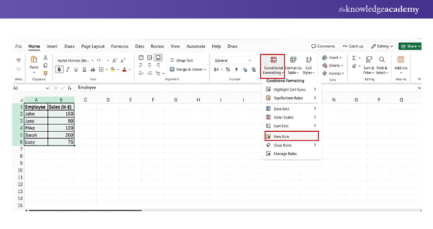
Step 2. Click on the Home tab and then select Conditional Formatting from the ribbon.

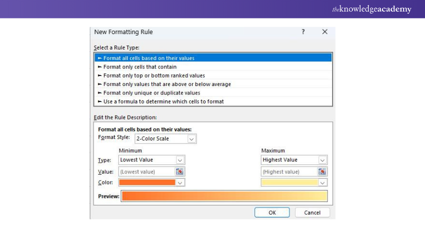
Step 3. Choose New Rule, and a dialogue box will appear with different rule types.

Step 4. Select a rule type, such as Format cells, that contains or uses a formula to determine which cells to format.

Step 5. Define the rule’s condition (e.g., cells greater than 100) and choose the formatting style (e.g., bold text, red fill).

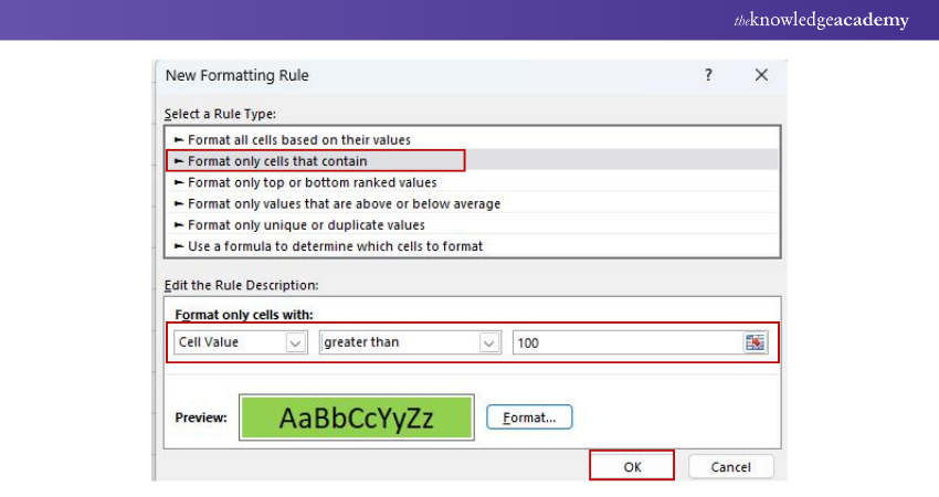
Step 6. Click OK to apply the rule.

2) How to Use a Preset Rule with Custom Formatting?

Excel offers several preset rules that can be quickly applied. To use a preset rule and customise it: 

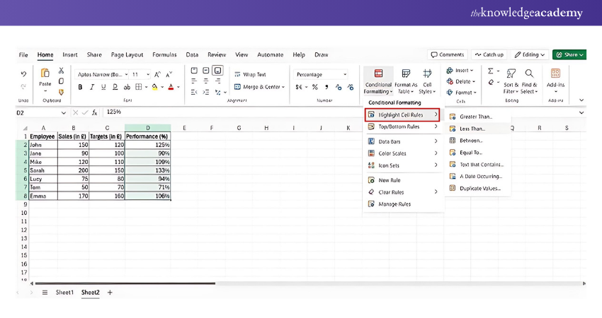
Step 1. Select the cells you want to format.

Step 2. Navigate to the Conditional Formatting menu and select Highlight Cells Rules or Top/Bottom Rules.

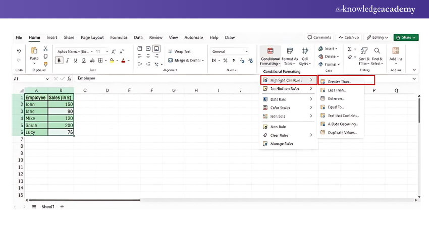
Step 3. Choose a rule (e.g., Greater Than, Less Than, or Duplicate Values).

Step 4. Input the required criteria (e.g., cells greater than 120).

Step 5. Click Custom Format to modify the preset’s format, such as changing the colour or font style.

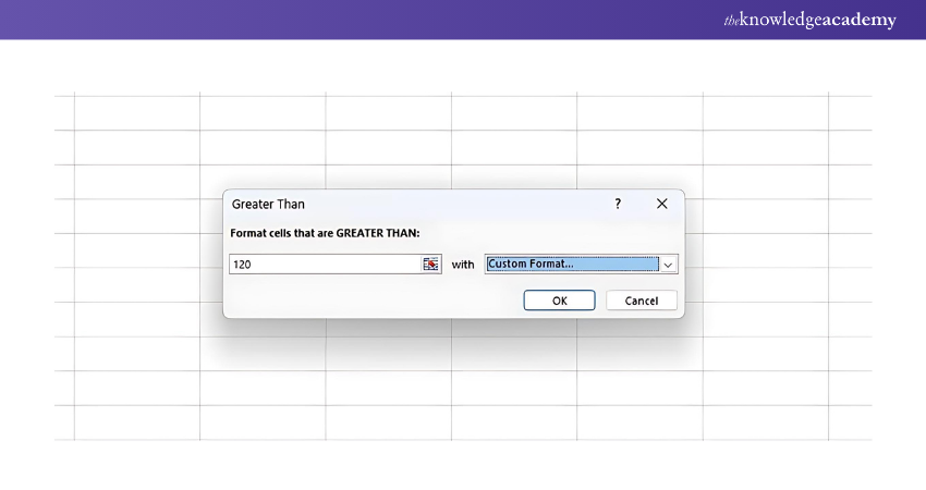
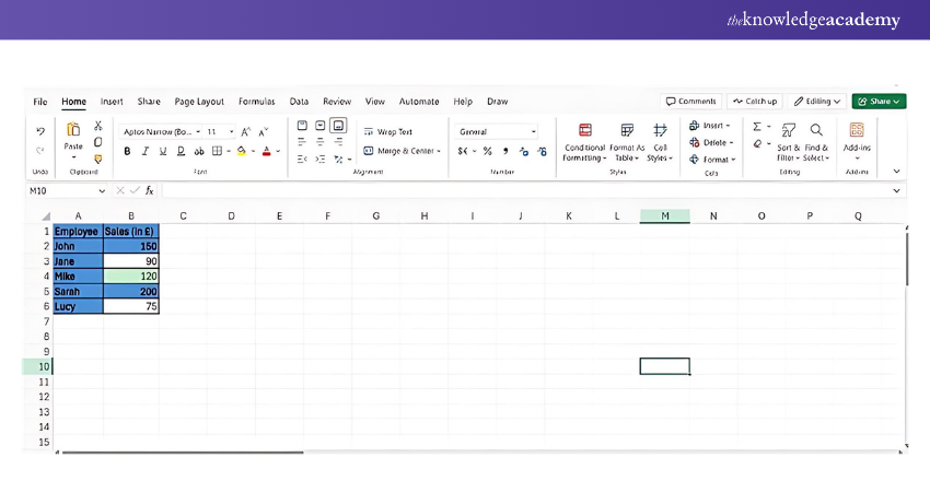
Step 6. Click OK to apply.

3) How to Edit Excel Conditional Formatting Rules?

Editing a Conditional Formatting rule in Excel is straightforward and allows you to quickly adjust or update existing rules to fit your changing data needs. Here's how to do it:

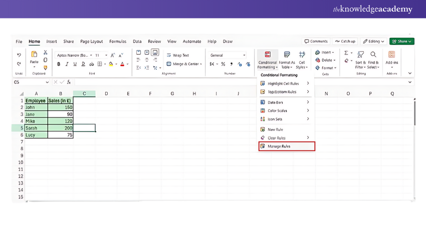
Step 1. Select the cells where the rule is applied.

Step 2. Open the Conditional Formatting menu and click on Manage Rules.

Step 3. In the Conditional Formatting Rules Manager dialogue, you’ll see a list of rules applied to the selected cells.

Step 4. Select the rule you want to alter and click Edit Rule.

Step 5. Make the necessary changes, such as adjusting the criteria or modifying the formatting style.

Step 6. Click OK to apply.

4) How to Apply Multiple Conditional Formatting Rules to the Same Cells?

Applying multiple rules to the same cells can help you layer conditions. Here’s how: 

Step 1. Select the range of cells.

Step 2. Apply the first Conditional Formatting rule as explained earlier.

Step 3. To add more rules, go to Conditional Formatting > New Rule and set up the additional rule.

Step 4. If necessary, use the Manage Rules option to set the order of the rules and adjust any conflicting rules by prioritising one over the other.

Advance your business insights – sign up for the Business Analytics With Excel Course and become an analytics expert!

Types of Conditional Formatting Rules and Styles

The following are the main types of rules and styles available in Conditional Formatting:

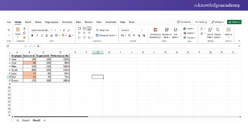
1) Highlight Cell Rules

a) Highlights cells based on specific criteria such as greater than, less than, equal to, or between certain values.

b) Ideal for identifying outliers, important thresholds, or specific conditions in your data.

 

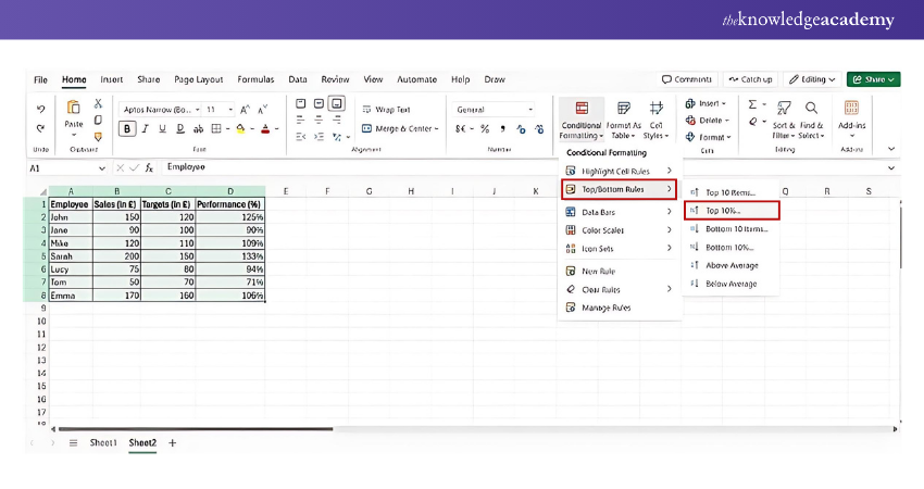
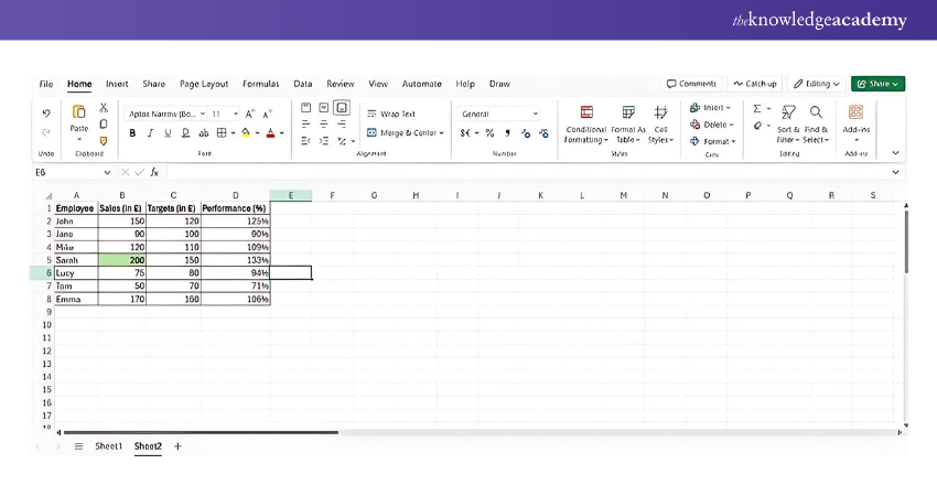
2) Top/Bottom Rules

a) Highlights the highest or lowest values in a dataset.

b) Can format the top 10%, bottom 10%, or a custom number of top/bottom values to highlight key performers or underperformers.

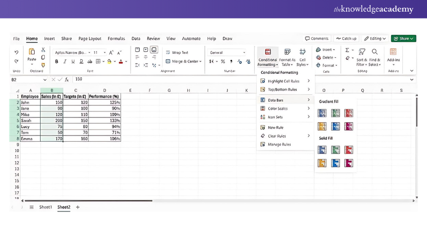
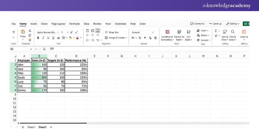
3) Data Bars

a) Visually represents cell values using a horizontal gradient bar.

b) The length of the bar reflects the cell's value relative to others, making it easy to compare data at a glance.

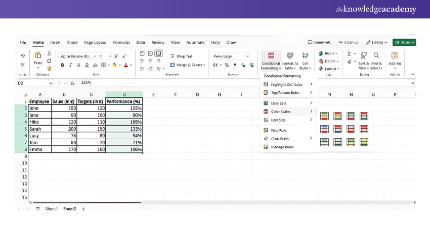
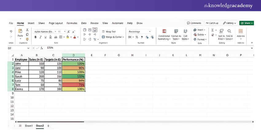
4) Color Scales

a) Applies a gradient of colours based on cell values.

b) Lower values may appear in red, middle values in yellow, and higher values in green, making it easier to spot trends or distributions.

5) Icon Sets

a) Uses symbols like arrows, traffic lights, or stars to represent data visually.

b) Provides an intuitive way to compare values and track performance or changes over time.

How to Copy Excel Conditional Formatting?

To copy Conditional Formatting from one cell or range to another in Excel, follow these steps: 

Step 1. Choose the cell with the formatting you want to copy: 

a) Select the particular cell or range of cells that already have the Conditional Formatting applied.

Step 2. Use the Format Painter tool: 

a) Go to the Home tab on the ribbon.

b) Click on the Format Painter icon (a paintbrush symbol). This tool copies the formatting, including Conditional Formatting, from the selected cell.

Step 3. Apply the formatting to other cells: 

a) Once you've activated the Format Painter, click on the cells or drag across the range where you want to apply the same Conditional Formatting.

b) The formatting will be applied, but the data will remain unchanged.

Alternatively, you can also use Ctrl + C (or Command + C on Mac) to copy the formatted cells and then use Paste Special > Formats to apply the formatting to other cells without affecting the data.

Enhance your Excel skills by learning Microsoft Excel VBA and Macro Training. Automate tasks and improve productivity now!

How to Clear Conditional Formatting Rules?

To remove Conditional Formatting from cells in Excel, follow these steps: 

Step 1. Select the cells: 

a) Highlight the range of cells where you want to clear the Conditional Formatting.

b) If you want to remove it from the entire worksheet, you can select the entire sheet by pressing Ctrl + A.

Step 2. Go to Conditional Formatting: 

a) Select the Home tab from the ribbon.

b) In the Styles group, select Conditional Formatting to open the dropdown menu.

Step 3. Clear Rules:

1) In the dropdown, select Clear Rules.

2) You will then be given two options:

a) Clear Rules from Selected Cells: This will remove Conditional Formatting from only the selected cells.

b) Clear Rules from Entire Sheet: This removes all Conditional Formatting from the entire worksheet.

Transform your accounting workflow with our Excel for Accounting Course - sign up now!

Conclusion 

Mastering How to Use Conditional Formatting in Excel unlocks the true potential of your data. With just a few clicks, you can turn ordinary spreadsheets into visual masterpieces, highlighting trends, spotting outliers, and making your analysis faster, smarter, and more intuitive. Watch your data come to life and tell its own story!

Enhance your Excel skills to new heights with our expert-led Microsoft Excel Course - register now and start excelling!