We may not have the course you’re looking for. If you enquire or give us a call on +08000201623 and speak to our training experts, we may still be able to help with your training requirements.
Training Outcomes Within Your Budget!
We ensure quality, budget-alignment, and timely delivery by our expert instructors.

Excel is one of the most powerful tools for Accountants. They use Excel to perform various financial tasks, create reports and make predictions. But often, Accountants spend a lot of time by manually inputting Data which is highly a time-consuming. Thus, the question is, how can Accountants find ways to perform task quickly without any costly errors? Excel Shortcuts are the saviours. Excel Shortcuts for Accountants make work more productive and streamline daily workflows. To learn the best Excel Shortcuts for Accountants, read this blog.
Table of contents
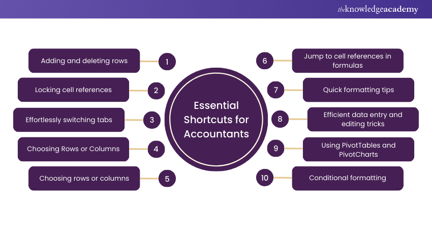
1) Essential Shortcuts for Accountants
a) Adding and deleting rows
b) Locking cell references
c) Effortlessly switching tabs
d) Choosing rows or columns
e) Adding totals to rows or columns
f) Jump to cell references in formulas
g) Quick formatting tips
h) Efficient data entry and editing tricks
i) Using PivotTables and PivotCharts
j) Conditional formatting
2) Conclusion
Essential Shortcuts for Accountants
There are several Excel Shortcuts for Accountants out there that you might not be aware of. Some help to navigate spreadsheets, create formulas, and analyse cell references. So, let’s find out some of these Shortcuts to help Accountants excel:

Adding and deleting rows
You can add and delete rows in Excel with simple Shortcut keys. After selecting rows and columns, use these Shortcuts:
a) Add: CTRL + “+” (plus key) or CTRL + SHIFT + “+” (plus key): To add rows or columns, hold down the CTRL key and press the “+” key.
b) Delete: CTRL + “–” (minus key) to delete rows or columns. Hold down the CTRL key and then press the “-” key.
Locking cell references
Locking cells helps to maintain the original cell reference. It is mainly used while working with lot of formulas. If you want cell reference to remain locked while copying and pasting a formula, add Dollar Sign ($) before the rows and columns. Manually adding the Dollar Sign might take some time. Hence, press F4 while typing a cell reference in a formula. This will insert $ symbols, resulting in locking the cell reference.
Effortlessly switching tabs
This Shortcut is useful when working on a spreadsheet with multiple tabs. Rather than using the mouse from one tab to another, use the below-mentioned Shortcuts:
a) Press and hold the CTRL key. Then, press the PAGE UP key to shift one sheet to the left, i.e. CTRL + PgUp.
b) Press and hold the CTRL key and the PAGE DOWN key to shift one sheet to the right, i.e. CTRL + PgDn.
Choosing rows or columns
This option is more convenient and efficient. It does not require mouse to choose rows and columns. Use the below-mentioned Shortcuts:
a) SHIFT + SPACEBAR: Hold and press the SHIFT key and the spacebar to select the row. To select multiple rows, hold the SHIFT key and use the up or down arrows to select the desired row(s).
b) CTRL + SPACEBAR: Hold and press the CTRL key and the spacebar to select the columns. To select multiple rows of columns, hold the SHIFT key and then use the right or left arrows to select the column(s).
Adding totals to rows or columns
You can save your time by not writing =SUM formula to sum up the cells. Instead, you can use ALT + “=” (equal key). To use this Excel Shortcut, Accountants can press Hold the ALT key, press the equal sign key, and then press Enter to complete an automatically inserted Sum formula.
Jump to cell references in formulas
This Shortcut is used when you are looking at a complicated formula or working on a sheet someone else worked. Instead of manually searching for the cell, use a Shortcut for it. The following are the Shortcuts you can use to jump to cell references:
a) CTRL + “[“: Select the cell with the formula you are working on. Hold the CTRL key and then press the “[” key to go to the first cell being referenced in the formula.
b) F5 + ENTER: After jumping to the referenced cell, you can go back to the original cell that has the formula by pressing the F5 key, then hit ENTER.
Enhance your knowledge of Charts in Excel with our Excel Training with Gantt Charts - sign up now!
Quick formatting tips
Formatting is essential for showing financial data. There are some Excel Shortcuts for Accountants to use when formatting worksheets. Let's find out:

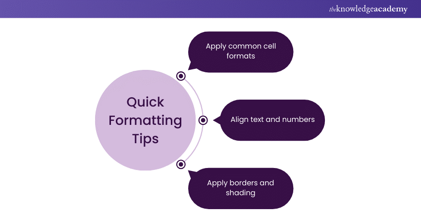
a) Apply common cell formats: Use CTRL + SHIFT + ~ for the general format, CTRL + SHIFT + ! for the number format, and CTRL + SHIFT + $ for the currency format (Indian Rupees).
b) Align text and numbers: To make your text align to the left and right, use CTRL + L, and CTRL + R. For making it centre alignment, use CTRL + E.
c) Apply borders and shading: To apply an outline border, Use CTRL + SHIFT + &. To remove the border, use CTRL + SHIFT + _. If you want to add shade, use ALT + H + H and choose the desired colour.
Efficient data entry and editing tricks
Accountants can often use Shortcuts to enter and edit data rapidly. These shortcuts are as follows:
a) Copy and paste: To copy and paste, use CTRL + C and CTRL + V. To paste special options, use CTRL + ALT + V.
b) Undo and redo actions: To undo and redo the last action, use CTRL + Z and CTRL + Y.
c) Clear and delete data: To clear the cell, press Delete. To delete a row or column, press CTRL + - after selecting.
Using PivotTables and PivotCharts
PivotTable is used to summarise, analyse, and present summary data. At the same time, PivotCharts complement PivotTables by inserting visualisations into the summary data. Here are the Shortcuts:
a) PivotTable: Select the data range and use ALT + N + V to add a PivotTable.
b) PivotChart: After creating a PivotTable, use ALT + N + Z to insert a PivotChart.
Enhance your knowledge of business analytics with our Business Analytics With Excel Course - sign up now!
Conditional formatting
Conditional Formatting makes the data visually appealing by highlighting values with colour. To apply conditional formatting, select the range and hit ALT + H + L to open the menu.
Sorting and filtering data
Sorting and filtering allow you to better analyse your data. It displays only rows that meet the criteria and hides that you do not want to display. To use this feature, follow these Excel Shortcuts:
a) Filters: Select a cell in your data range and Ctrl + Shift + L to add filters.
b) Sort: Press ALT + A + S + A or an ascending sort and Alt + A + S + D for a descending sort.
Crafting and applying templates
It is a pre-built spreadsheet or workbook that is already formatted and organised. Here are the Shortcuts for crafting and applying templates:
a) Save workbook as a template: Choose File > Save As > Browse and select Excel Template (*.xltx) as the file type.
b) Use custom template: choose File > New > Personal and select the preferred template.
Using and recording Macros
It is a process where Excel records every task and action that can be run many times. To Save Accountants valuable time, they can follow these Shortcuts:
a) Record Macro: Use ALT + F11 to open the Visual Basic for Applications (VBA) editor. Choose the record macro to perform the actions, and then click Stop Recording.
b) Run Macro: Use Alt + F8 to open the dialogue box. Select the macro, and then click Run.
Conclusion
We hope this blog made you aware of the top Excel Shortcuts for Accountants. By incorporating these keyboards Excel Shortcuts, Accountants can notably improve accuracy and the quality of the reports. We hope by using these Shortcuts you become a master in MS Excel.
Master your Excel shortcut skills with our Microsoft Excel Training - register today!
Frequently Asked Questions

PivotTable is used to summarise, calculate, and analyse data for comparison, patterns and trends. To create a PivotTable, select the data range and press ALT + N + V.

PivotTable is used to summarise, calculate, and analyse data for comparison, patterns and trends. To create a PivotTable, select the data range and press ALT + N + V.

The Knowledge Academy takes global learning to new heights, offering over 30,000 online courses across 490+ locations in 220 countries. This expansive reach ensures accessibility and convenience for learners worldwide.
Alongside our diverse Online Course Catalogue, encompassing 17 major categories, we go the extra mile by providing a plethora of free educational Online Resources like News updates, Blogs, videos, webinars, and interview questions. Tailoring learning experiences further, professionals can maximise value with customisable Course Bundles of TKA.

The Knowledge Academy’s Knowledge Pass, a prepaid voucher, adds another layer of flexibility, allowing course bookings over a 12-month period. Join us on a journey where education knows no bounds.

The Knowledge Academy offers various Microsoft Excel Training & Certification Course, including Microsoft Excel Masterclass, Excel for Accountants Masterclass, and Business Analytics With Excel Masterclass. These courses cater to different skill levels, providing comprehensive insights into Excel methodologies.
Our Office Applications Blogs cover a range of topics related to Microsoft Excel, offering valuable resources, best practices, and industry insights. Whether you are a beginner or looking to advance your Excel skills, The Knowledge Academy's diverse courses and informative blogs have you covered.
Upcoming Office Applications Resources Batches & Dates
Date
 Excel for Accounting Course
Fri 17th Jan 2025
Fri 21st Feb 2025
Fri 4th Apr 2025
Fri 6th Jun 2025
Fri 29th Aug 2025
Fri 24th Oct 2025
Fri 26th Dec 2025


 Top Rated Course


 If you wish to make any changes to your course, please


