We may not have the course you’re looking for. If you enquire or give us a call on +44 1344 203 999 and speak to our training experts, we may still be able to help with your training requirements.
Training Outcomes Within Your Budget!
We ensure quality, budget-alignment, and timely delivery by our expert instructors.

Microsoft Excel, a popular spreadsheet software, has many functionalities. You can use the Percentage Formula in Microsoft Excel to calculate the 'per cent' value of a figure. The Latin word "percent" signifies "by 100". The basic formula used to calculate percentage is the numerator divided by the denominator. Next, the result is multiplied by 100. Fortunately, the advent of Excel has made percentage calculation even more straightforward.
Excel helps you calculate percentages easily by entering the value and percentage in your spreadsheet. Some Excel formulas allow you to calculate changes in percentage or percentage of totals of the same item entered multiple times.
Excel simplifies using percentages by applying advanced and basic formulas automatically. Consequently, Excel finds its use among at least 66% of office workers each hour. The objective of Excel is to save the time of office workers. This will help you understand how to use the Percentage Formula in Excel. We'll be covering the following topics in this blog:
Table of Contents
1) How to use Percentage Formula in Excel?
2) How to use simple Percentage Formulas in Excel?
3) Example 1: How to calculate a change in percentage?
4) Example 2: Calculate Percentage increase or decrease in Excel
5) Example 3: Percent change between 2 columns
6) Example 4: Percent change between rows
7) Example 5: Estimating total Percentage in Excel
8) Example 6: Calculating the Percentage difference between two numbers
9) Example 7: Parts of the total are in multiple rows
10) Example 8: How to increase/decrease a number by percentage
11) Key takeaway
12) Conclusion
How to use Percentage Formula in Excel?
The basic mathematical formula for Percentage is (Part/Whole*100). In contrast, Excel's Percentage Formula doesn't include '*100'. Excel can calculate the Percentage automatically once you have applied the Percentage format to each cell. So, when calculating a Percentage in Excel, you'll no longer have to multiply the result of the fraction by 100.

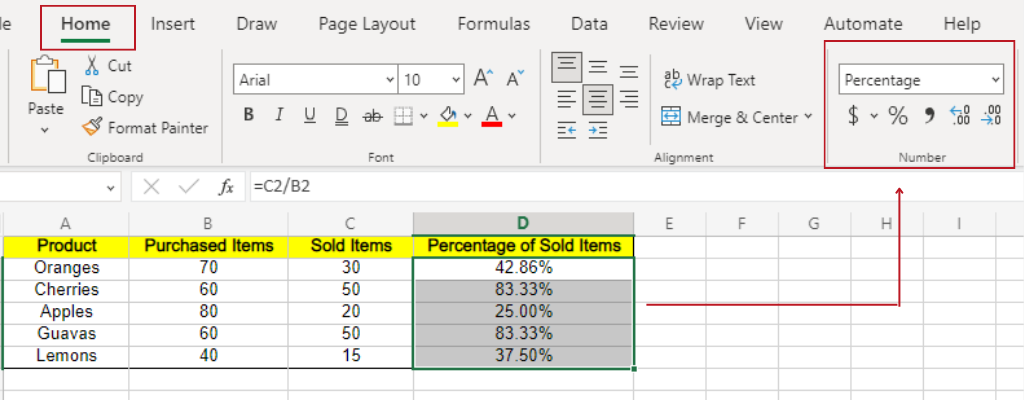
Let's see how to use this formula with the help of a real-life example. Suppose column A includes the list of "Purchased items", and column B consists of the list of "Sold items". To derive the Percentage of sold items, you can follow the following steps:
Select cell D2 and insert the formula =C2/B2.

Select the Home tab > Number group and select the Percent button.
This will convert the decimal fraction to a percentage. You can also increase or decrease the decimal places if required.
In the following image, column D represents a Percentage of delivered items. Here, we have converted the decimal value into a percentage.
How to use simple Percentage Formulas in Excel?
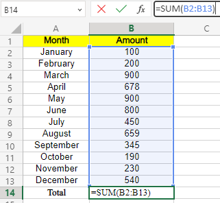
You can also use the simple percentage formula to ease your daily calculation tasks. Firstly, you’ll have to add the total expenses.
Step 1: You need to derive the sum of all amounts. To do this, you must enter the following formula =SUM(B2:B13) in B15.
Step 2: Calculate the percentage of the total or the simple percentage for January in Column C. for example, For January, you can use the formula =(B2/B14)*100. I.e. =(Amount/Total)*100.
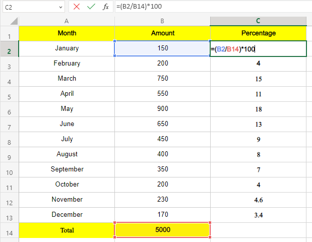
Tip: If the resultant value is represented in decimal format, you must convert it into a percentage. You can change this value into a percentage by clicking on the percent symbol.
Become an expert in visualisation, register for Microsoft Excel Courses
Example 1: How to calculate a change in percentage?
The two popular formulas you’ll be using when calculating percentages in MS Excel are the Percentage of change and the Percentage of growth. To calculate the difference between the original value of column B and column C is:
Percentage Change= (C-B)/B
Calculation of percentage of change between two columns.
The value of column B shows the original value that hasn’t been changed. For example, when we compare the sales of two months, April and May, the sales in April represent the original value of sales. Let’s take a look at the following example to learn how to calculate percentage growth:
=(C2-B2)/B2
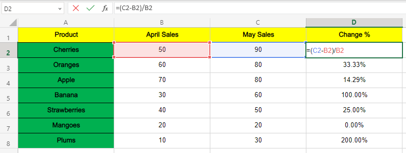
Note: Calculation showing an increase in the percentage of sales using an Excel formula
Percentage of growth =(B3-B2)/B2
Calculation of percentage growth between two distinct rows
You can use the Excel spreadsheet to track the total number of sales every month. Here, you can calculate an increase and decrease in growth and represent it in percentage. The data included in two rows are used to estimate the changes in sales every month. For example, the sales that take place every month are included in column B.
Similarly, the percentage of growth calculated is entered in column C. Enter the sales data in B2 in January. Next, you can calculate the increase in sales for February by selecting cell C3. To derive this value, you’ll have to enter the formula inside cell C3=(B3-B2)/B2
Next, you can use this formula in the following rows commencing from C4. The % of growth in the Excel spreadsheet is shown as:
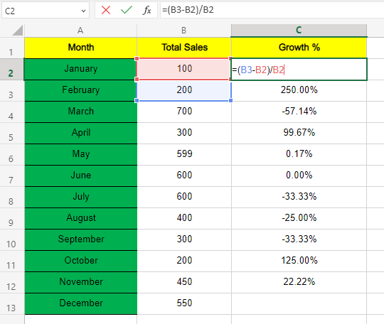
Note: When calculating the growth % in Excel, you can leave C2 or the first row in Column C blank. You cannot include C2 because it is not being compared with any of the other values. In our example, the sales figure for January isn’t being compared to the former month.
Build your career as a Data Analyst - sign up for Data Analysis Training using MS Excel!
Example 2: Calculate Percentage increase or decrease in Excel
You can follow a few simple techniques to calculate percentages in Excel. In our example, we've used a sheet with a list of travel expenses in different months. Here, you’ll be able to understand how the % can change due to an increase or decrease in prices for each month.
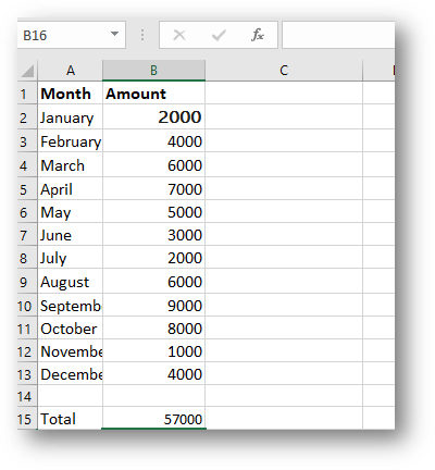
Step 1: Suppose you expect an increase in your travel expenses by 7 percent. It’s important to note that Excel allows you to enter percentages in the form of a decimal or a percent sign. For example, when you can include thirty percent in the spreadsheet by entering 0.3 or 30%. Excel’s formatting function will consider these two values same.
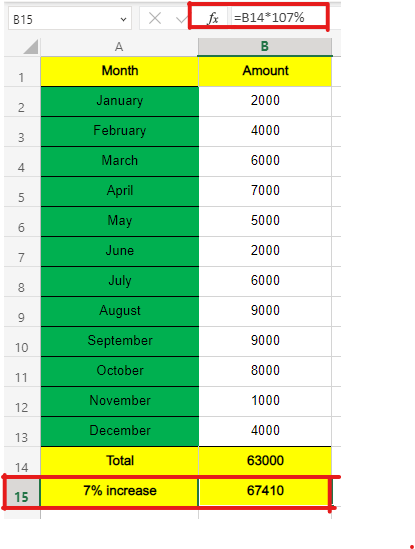
In B14, enter:
= B14* 1.07
Or, if you want, you can enter it in the following format:
=B14*107%
The result derived is:
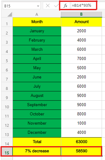
Step 2: Suppose you expect your travel expenses to decrease by 7 percent. Here, you can calculate the amount in numbers. You can use the below mentioned-steps to calculate the estimate in figures.
In B14, enter:
=B14*93%
Or, you can also enter the value as:
=B14*.93
The result derived is:
Example 3: Percent change between 2 columns
Let’s say you want to calculate the price difference between two columns; we can do this using simple formulas. In this case, we will find the Percentage difference between columns B and C using the following methods. Conditional Formatting can be applied to highlight the cells that meet certain criteria, making it easier to apply the Percentage Formula.
Method 1
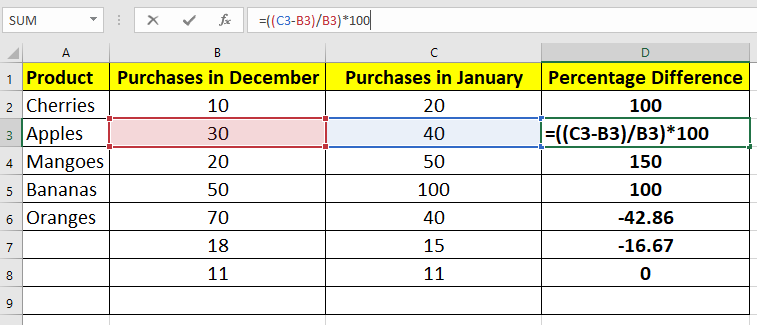
Percentage Difference formula =((C2-B2)/B2)*100
Step 1: Enter this formula in an empty cell next to the columns for which you want to find the difference. Here, we have entered our formula in cell D2, which is empty and close to the other columns.
Step 2: Drag the formula pasted in cell D2 and drag it down further to find the Percentage difference for all the cells with data.
Method 2
Percentage Difference formula =(C2-B2)/B2
Step 1: Select all the cells in column D and change the numbering format from general to Percentage on the home tab.
Step 2: Enter the above formula in an empty cell.
Step 3: Drag and drop the formula to find the Percentage difference for other rows.
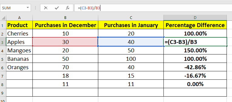
It is as simple as that; you can use any of the above two methods to determine the Percentage difference between 2 columns.
Example 4: Percent change between rows
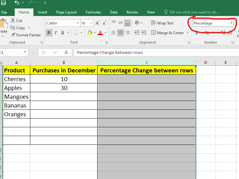
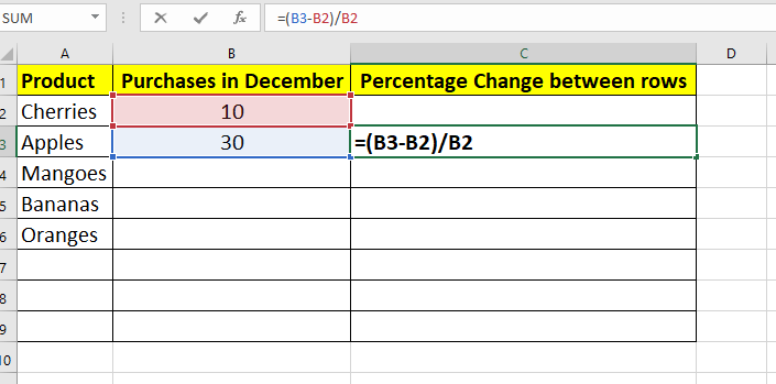
Formula to find the Percentage difference between rows =(B3-B2)/B2
Step 1: Enter the entire column where you want to paste the formula and change its formatting to Percentage from the home tab.
Step 2: Enter the formula in an empty cell
Step 3: Drag and drop the formula down to find out the value for all the cells.
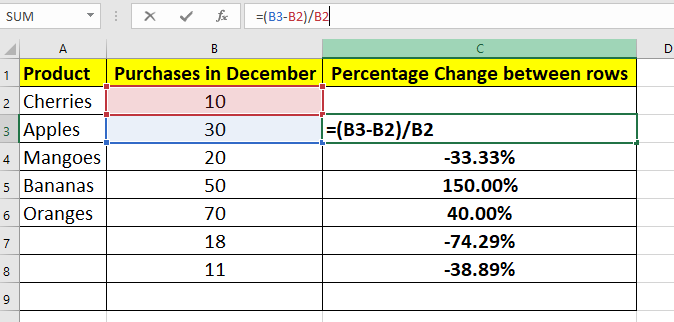
The final result would look something like this
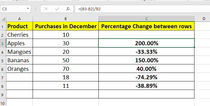
There you go; we have now calculated the Percentage difference between two rows with a simple formula.
Example 5: Estimating total Percentage in Excel
In the above example, we learn how to calculate an increase or decrease in percentage. However, using Excel is also helpful in making several complex calculations to find the percentage of the total.
Step 1: Calculate the percentage of a total at the end of the table
This step is helpful if the retailer wants to know the total number of products he purchased. Similarly, the retailer can evaluate the part (%) of the total purchase amount attributed to a particular product. Excel calculates the part of the total percentage that a specific amount represents.
To calculate this, firstly, we will have to add the number of items in cell B10 by using the formula =SUM (B2:B9). In the right column or column C, we will enter an Excel formula to calculate the total percentage represented by each product. Secondly, to calculate this, we’ll have to use the formula =B2/B10, B3/B10, B4/B10, etc. Also, you can select the value by clicking on the mouse button. Next, you can convert decimal numbers into percentages by clicking on %.
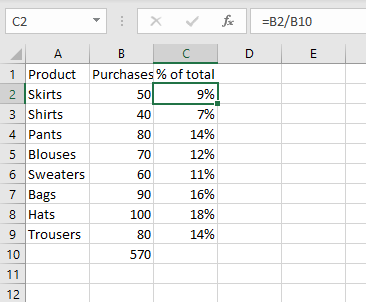
Note: The value of B10 doesn't change here. However, the other values can change as per the formula used in the spreadsheet.
Step 2: Calculate the percentage of the total in different rows
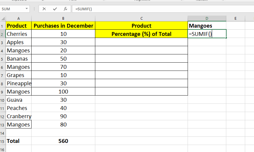
Sometimes a retailer has to maintain multiple rows to represent the quantity of the same product. Let's say the retailer wants to calculate the total percentage represented by a particular product.
In this case, the retailer can apply the SUMIF formula. The SUMIF formula helps to derive the sum of the values that can match your chosen criteria. When the SUMIF formula is combined with the formula for calculating percentages, the Excel formula is written as:
=SUMIF(range, criteria, sum_range)/total
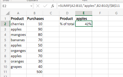
Note: The SUMIF formula in MS Excel helps to calculate the total percentage a particular product represents. The SUMIF formula is used to add the values under your chosen criteria.
We have chosen the criteria “apples” in our example in E1. The sum of values that we want to derive is listed under column B. Similarly, the product names we want to select automatically are listed under column A. So, you can use any of the two formulas
=SUMIF(A2:B10, “apples”, B2:B10)/$B$11 or SUMIF (A2:B10, E1, B2:B10)/$B$11
Sign up and learn the top 10 Excel shortcuts and how to apply percentage formula in Excel with our Microsoft Excel Courses
Example 6: Calculating the Percentage difference between two numbers
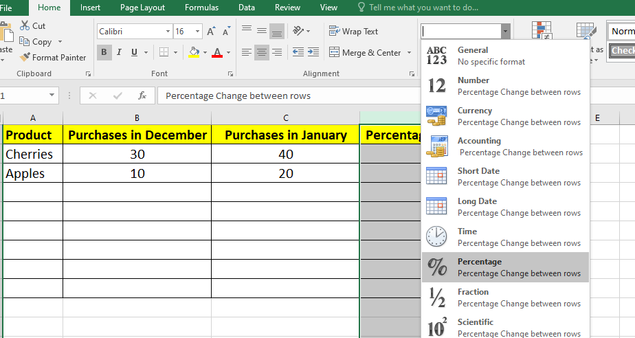
Step 1: Select the column where you want to find the Percentage change difference between two numbers and change its formatting to a Percentage similar to the image shown below.
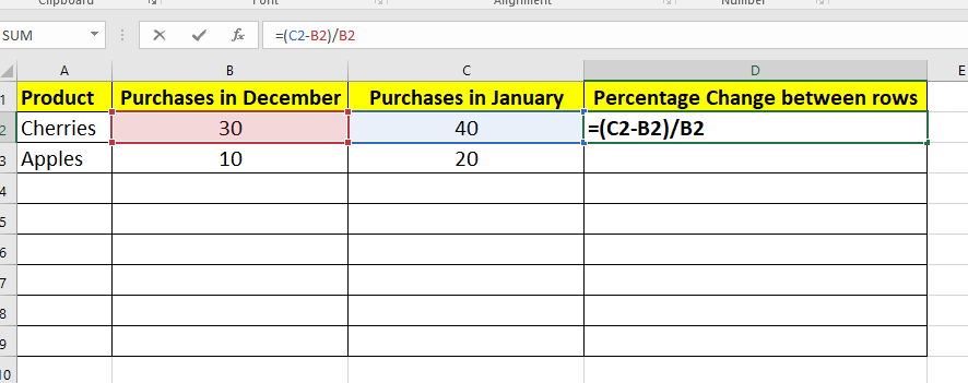
Formula to find the Percentage difference between two numbers =(C2-B2)/B2
Step 2: Enter the formula in the empty cell where you want the values to be shown
Step 3: Copy the formula to all the cells using the fill handle.
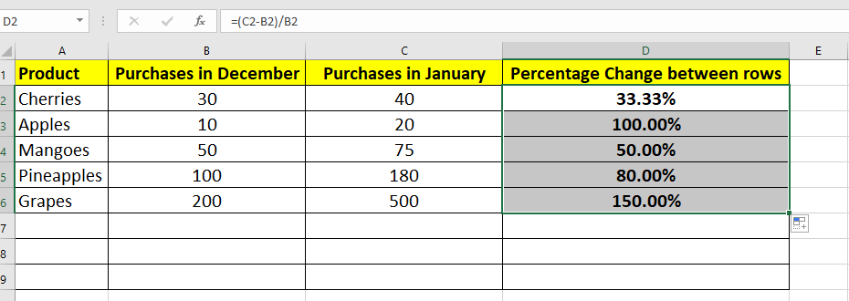
Now we have calculated the Percentage difference between the two numbers.
Example 7: Parts of the total are in multiple rows
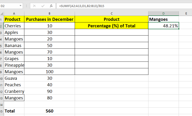
To find out the value for parts of the total which are in multiple rows, we can use the following formula:
Formula =SUMIF(range, criteria, sum_range) / total
Step 1: Make sure the cell where you want the Percentage value has a Percentage format on the home tab.
Step 2: Next, enter the formula in an empty cell. For example, we are using Cell D2
.
Step 3: Select the ranges for which you want to find the Percentage values.
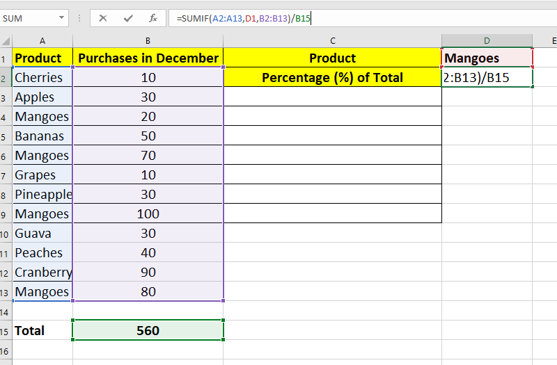
Now let’s find out the final value, as shown in the image below:
Example 8: How to increase/decrease a number by percentage
Calculating the increased and decreased value by Percentage is super simple. We are going to find them out with examples.
How to increase a number by percentage?
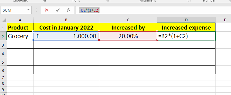
Welcome to 2023, where inflation is skyrocketed in many countries on the planet. To make this interesting, let’s use a simulated example highlighting the impact of inflation right now.
We can use the following formula to increase a number by a percentage:
Formula to Increase = Number * (1 + Percentage value)
Let’s say the monthly average grocery price in January 2022 was 1000 GBP; we will calculate the value for a 20 per cent increased grocery cost for the current year.
We can use the following formula to increase a number by a percentage:
Formula to Increase = Number * (1 + Percentage value)
Here in our example, the formula =B2*(1+C2)
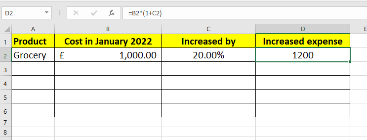
So, when we increased the number by 20 per cent, the value changed to 1200 GBP.
How to decrease a number by percentage?
For the prospect of a brighter future, let’s assume that inflation will cool down in the current year and decrease by 20 per cent.
To decrease a number by a percentage, we can use the following formula:
Formula to Decrease = Number * (1 – Percentage value)
Here in our example, the formula =B2*(1-C2)
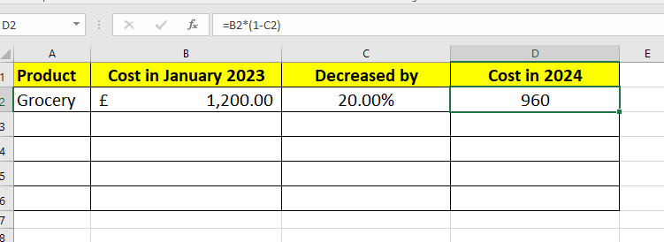
Now the cost of 1200 GBP is reduced to 960 GBP for 2024; hopefully, something like this happens in real life too!
Key takeaways
a) To remove the percent error, you can use the IFERROR function.
b) The percentage is represented as a proportion per 100.
c) You’ll have to divide the numerator by the denominator to calculate the percentage. Then multiply the result by 100.
d) Usually, Excel users get a percentage value in the form of a decimal. Next, Excel users can convert it by using the % form.
e) To change the resultant data into percentage form, users can use Excel Shortcuts and enter the shortcut command Ctrl+Shift+% in Microsoft Excel.
Conclusion
We hope after reading the blog, you now understand how to use the Percentage Formula in Excel. Users who find it challenging to calculate percentages in Excel can follow the basic steps mentioned above. When familiar with these basic Excel Formulas and Functions, you’re more likely to derive an accurate result.
Learn how to use advanced formulas in MS Excel - Sign up for Microsoft Excel Expert!


 Top Rated Course


 If you wish to make any changes to your course, please


