We may not have the course you’re looking for. If you enquire or give us a call on +800 312616 and speak to our training experts, we may still be able to help with your training requirements.
We ensure quality, budget-alignment, and timely delivery by our expert instructors.

Microsoft Excel is widely considered as one of the best tools preferred and commonly used in every industry to organise, simplify, structure, and manage data across organisations. This application is probably used by every professional out there to generate reports and business insights. Therefore, it is crucial that you know the Basic Excel Formulas and Functions and learn how to utilise them for your projects.
There are numerous keyboard shortcuts available in Excel that can be used to increase the organisation's productivity. A decent knowledge of Microsoft Excel can land you in jobs mostly related to the financial sector or accounting. This blog has discussed some of the most important Basic Excel Formulas and Functions to help you navigate this application. Read further to know more!
Table of Contents
1) Excel Formulas and Functions
2) List of Basic Microsoft Excel Formulas
a) SUM
b) MAX & MIN
c) AVERAGE
d) COUNT
e) TRIM
f) IF
g) POWER
h) CEILING
i) FLOOR
3) Conclusion
Excel Formulas and Functions
Microsoft Excel is a highly popular tool for data management and analysis, frequently used to generate analytical reports, uncover business insights, and store operational records. To carry out basic calculations or Data Analysis, Excel formulas are essential.
Even the most basic Excel formulas enable you to manipulate data types such as text, numbers, and dates. The Microsoft Excel Formulas Guide also shows how you can apply various functions like IF-ELSE statements, find and replace features, and specialized formulas in areas such as mathematics, trigonometry, finance, logic, and engineering.
Unlike traditional programming languages, working with Excel formulas is simple. All you need to do is input the formula name and the required arguments—there’s no complexity involved. Excel also offers a user-friendly interface that assists you in adding formulas, making it accessible to everyone, regardless of technical expertise.
List of Basic Microsoft Excel Formulas
A Formula helps in the calculation of values in a selected range of cells or just a cell. Formulas in Excel can contain functions, references, operators and constants (a value that isn’t calculated).
1) SUM
The SUM() function, as its name implies, calculates the total of a selected range of cell values by performing the addition operation. Below is an example:
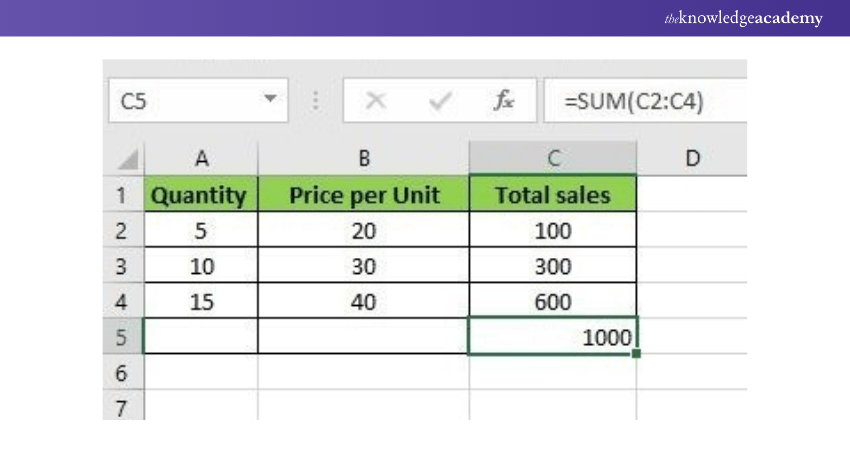
As shown in the figure, to determine the total sales for each unit, we simply entered the function “=SUM(C2:C4)”. This automatically adds the values 100, 300, and 600, and the result is stored in cell C5.
2) MAX & MIN
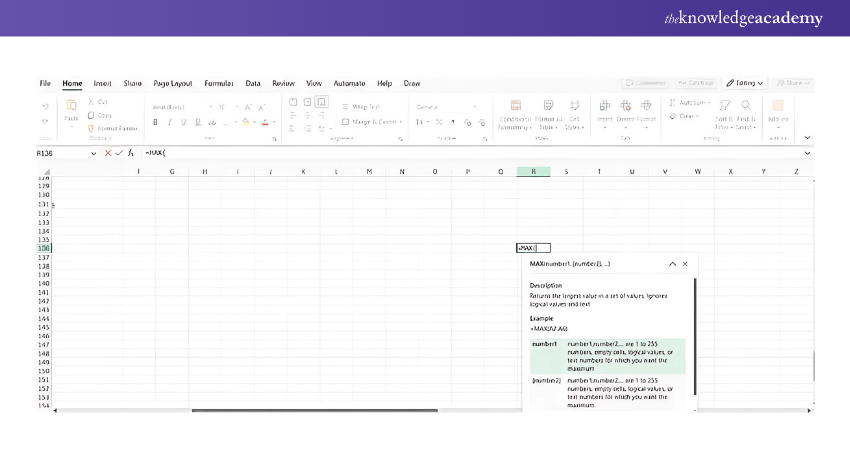
The MAX and MIN functions in Excel are designed to quickly identify the highest and lowest values in a range of numbers. These functions are particularly useful when working with large datasets, as they eliminate the need for manually scanning through the data to find the extremes.
For example, to find the largest value in a dataset, you would use the MAX function as follows:
=MAX(B2:B6)
Similarly, to find the smallest value in the same range, you would use the MIN function:
=MIN(B2:B6)
3) AVERAGE
The AVERAGE Function is used to derive simple Averages for the data. It follows the syntax:
=AVG(num1, [num2], …)
The following image is an example of using the AVERAGE Function to calculate the average of a selected set of values or numerical:
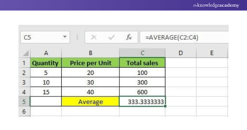
The above table shows that by entering the Function “=AVERAGE(C2:C4)”, it is possible to figure out the average of a specified set of values (C2 to C4 in this case).
4) COUNT
The COUNT Function is used to Count the numeric values given in a certain cell range. It follows the syntax:
=COUNT(value1, [value2], …)
The following is an image that shows how the COUNT Function works with a string of text values and numerical values:
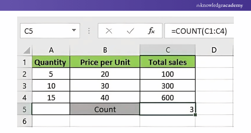
This image showcases the use of the COUNT Function to obtain the number of values that are numerical in nature. The result is obtained upon entering the Function “=COUNT(C1:C4)”, because all the values from C1 to C4 were the selected values.
Boost your Tally efficiency with the Tally Shortcut Keys PDF. Download it now and start mastering essential shortcuts for faster operations.
5) COUNTA
The COUNTA Function counts all the cells in the given range regardless of the type of cells. It follows the syntax:
=COUNTA(value1, [value2], …)
The following image showcases the use of the COUNTA Function:
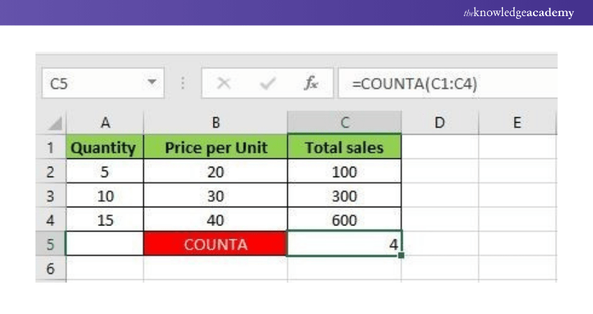
This image shows us how to use the COUNTA Function to obtain the result of the total number of values regardless of their type. Here, the Function “=COUNT(C1:C4)” has been used to count all the values from cell C1 to cell C4.
6) TRIM
The TRIM Function removes all the empty spaces in the cell selected. It can operate in only one cell at a time; it ensures that your functions do not return with errors due to the extra spaces in the data. It follows the syntax:
The following image shows us the correct usage of the TRIM function:
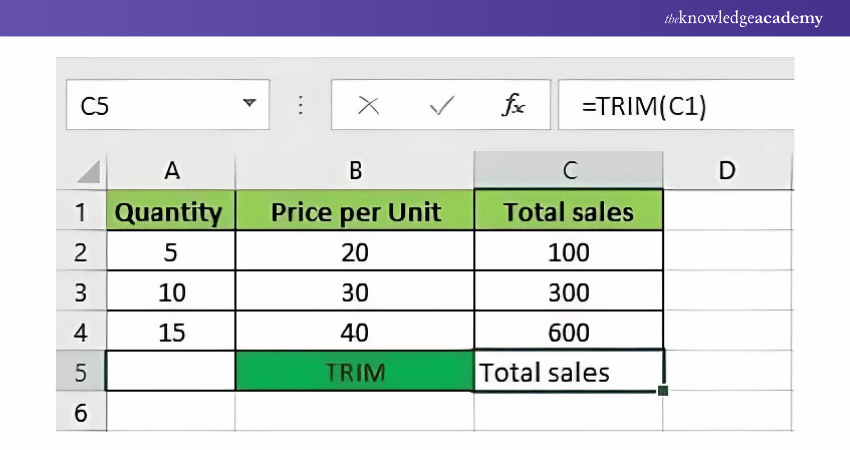
Here, the TRIM Function has been used on the cell with the value ‘Total Sales’. The Function “=TRIM(C1)” has provided us with the text in cell C1 without any extra spaces.
7) IF
The IF() function in Excel evaluates a given condition and returns a specific value if the condition is TRUE, and another value if it is FALSE. This makes it an essential tool for conditional logic in Excel.
For instance, in the example below, we check whether the value in cell A2 is greater than 5. If it is, the function will return the message “Yes, 4 is greater.” If the value is not greater than 5, it will return “No.”
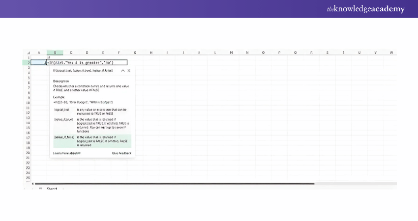
In this case, since 4 is not greater than 5, the function will return "No."
Another commonly used function is IFERROR. This function is useful for handling errors in calculations. If an expression results in an error, IFERROR will return a custom message or value. Otherwise, it will return the result of the expression. Similarly, the MROUND Function in Excel can be used to round numbers to a specified multiple, helping to ensure accurate and error-free calculations.
For example, if you attempt to divide 10 by 0 (which is mathematically invalid), the formula would return an error. Using IFERROR, you can instruct Excel to return a message like "Cannot divide" instead of displaying the error.
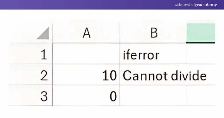
Both IF and IFERROR functions simplify logical operations and error handling, making Data Analysis more efficient and user-friendly.
8) POWER
The POWER Function in Excel is a mathematical function. It produces the result of a number raised to a specific power. It works with the base and the exponent. Initially, we used the “^” symbol to apply exponents in Excel. While this method works, it's not the most efficient or flexible approach for performing power calculations.
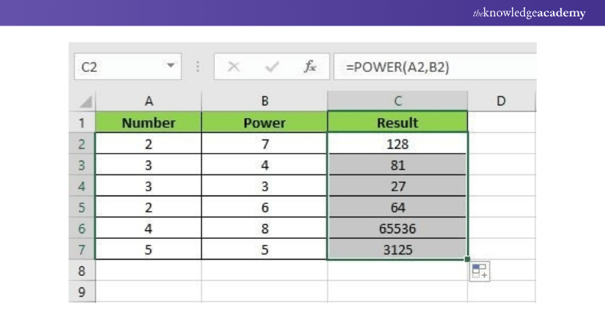
The image above contains values for the base number and power. Using the Function “=POWER(A2,B2)”, the values A2 and B2 were selected as the base number and power, respectively, to obtain the desired result. Upon dragging down the cell with the Function, the condition is also applied to the remaining cells.
A better alternative is to use the POWER() function, which allows you to easily square, cube, or raise a number to any specified power within a cell. This formula is more robust and preferred for complex power operations in Excel.
9) CEILING
The objective of the CEILING Function in Excel is to round up to the nearest multiple of a given number. It operates with instructions on the number that is to be rounded and the multiple to use when rounding. It follows the syntax:
=CEILING(number, significance)
The following image shows an example of using the CEILING Function in Microsoft Excel:
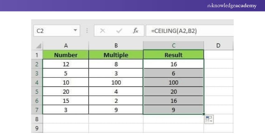
The image displayed above shows how using the Function “=CEILING(A2,B2)” has helped provide our desired result. The values provided in cells A2 and B2 have been used to formulate the rounding up of the number in A2
10) FLOOR
Contrary to the CEILING Function, the FLOOR Function in Excel is used to round down to the nearest multiple of the provided number. It requires the number to be rounded and the multiple to refer to the rounding while operating. It follows the syntax:
=FLOOR(number, significance)
The following image is an example of using the FLOOR Function in Microsoft Excel:
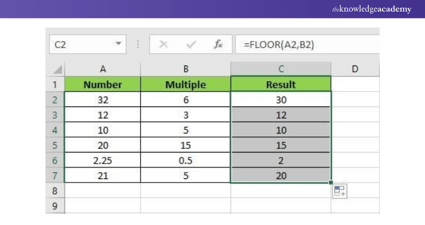
This image shows the steps required to round down a given number to the nearest multiple. According to the values provided in the above cells, the Function used to obtain the desired result is “=FLOOR(A2,B2)”.
11) LEN
The LEN Function in Excel helps in returning the length of a specified text string as the number of characters. It also helps count characters in numbers, spaces, and even special characters. The syntax it follows is:
=LEN(text)
The following image is an example of using the LEN Function in Microsoft Excel:
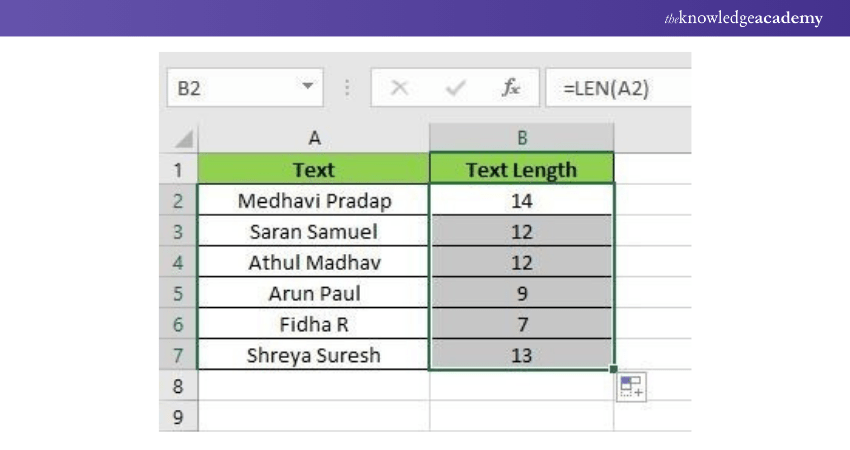
The image above shows us the correct way to use the LEN Function. By using the Function “=LEN(A2)”, you can figure out the length of the text or values provided in the cell ‘A2’. The text length of the following cells is also displayed above.
Build your career as a Data Analyst and learn the usage of Microsoft Excel for Data Analysis purposes with Data Analysis Training using MS Excel Training.
12) UPPER, LOWER, PROPER
The UPPER Function helps in the conversion of text strings to uppercase. Similarly, the LOWER Function helps in the conversion of a selected text string to lowercase. The PROPER Function converts text from a selected text string to the proper case. In the proper case, the first letter of each word is capitalised, and the rest is in lowercase.
The syntax for UPPER Function: =UPPER(text)
The syntax for LOWER Function: =LOWER(text)
The syntax for PROPER Function: =PROPER(text)
The following image is an example of using the UPPER Function:
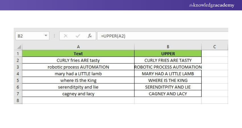
The image shows some random text that was conditioned to produce results in uppercase. Using the Function “=UPPER(A2)”, you can obtain results which are fully in uppercase. The same condition is applied to all the text values.
The following image is an example of using the LOWER Function:

The image above shows an example of converting certain words to lowercase. The Function “=LOWER(A2)” has been used to convert the text values in A2 to lowercase. The same condition has been applied to the rest of the values.
The following image is an example of using the PROPER Function:
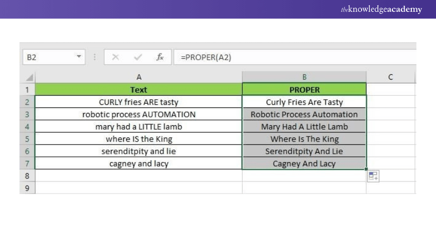
The above image shows some random words being given the PROPER Function. It converts the given data into the appropriate result. The Function “=PROPER(A2)” was used to obtain result on text in cell A2.
13) INDEX MATCH
The INDEX and MATCH Function, as the name suggests, is a combination of the INDEX and the MATCH functions. The INDEX Function is a flexible FORMULA that provides the value of a specified location within a range.
Formula: =INDEX(C3:E9,MATCH(B13,C3:C9,0),MATCH(B14,C3:E3,0))
The following image is an example of using the INDEX and MATCH Function:

In the above image, we have used data based on the names of salespeople in a company and listed their respective sales for each month. The objective here is to find the sales number for the month of February for the salesperson ‘Jackson’. As INDEX is used to retrieve a value within a range, we provide the values of B2:D7 with row 4 and column 2.
The MATCH Function is used to find the position we require. Nesting the MATCH Function within the INDEX, we use the final Formula “=INDEX(B2:D7,MATCH("Jackson",A2:A7,0),2)”.
14) IF Combined with AND / OR
The IF AND/OR Formula is a result of the combination of two logical functions. The use of the AND Function characterises the presence of multiple conditions. This Formula can be used for any set of values.
Formula: =IF(AND(C2>=C4,C2<=C5),C6,C7)
The following is an image that showcases the usage of the IF AND Formula with an example:
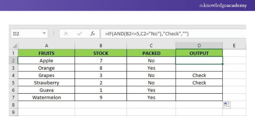
Here, data regarding fruits, the number of fruits in stock, and whether they are packed or not is provided. The IF AND Function is applied using a combination of less than equal to (<=) and the equal to (=) text Function. The Formula used in this situation is:
=IF(AND(B2<=5,C2="No"),"Check","")
As the “Output” column shows, the results on each cell follow the same condition. There are two observations made from the results in the last column:
a) The IF Function presents the result of “Check” only if the arguments entered in the AND Function are “true.”
b) The IF Function presents a blank string if either of the arguments in the AND Function is “false” or both the arguments are “false”.
15) OFFSET combined with SUM or AVERAGE
The OFFSET Function in Microsoft Excel returns the value of a cell or a range of adjacent cells from the reference point. The reference point is the starting cell that has been provided to a Function as an argument.
Formula: =SUM(B4:OFFSET(B4,0,E2-1))
The following image is an example of using the OFFSET Function with the SUM Function:

The image displayed above holds the data on five stock names and their maximum and minimum returns. The objective is to use the SUM Function on the maximum returns of the stock. Here, we use the OFFSET combined with SUM Function in the Formula:
=SUM(OFFSET(B2,0,0,6,1))
In this Formula, B2 is the reference point. The mention of two zeroes is to signify that the OFFSET Function won’t move up, down, right, or left. The height (number of rows) of the considered range is 6. This means that the OFFSET Function sums six rows beginning from cell B2. This includes the range B2:B7. The width (number of columns) argument is 1. This implies that the OFFSET Function will sum the values of column B.
16) SUMIF and COUNTIF
The SUMIF Function provides the sum of cells that are based on a single condition. Criteria or conditions can be added to text, numbers, and even dates. The COUNTIF Function in Excel is used to count the number of cells that fulfil a condition. It can also be used on text, numbers, and dates.
a) SUMIF
The SUMIF Function is a widely used Function in Excel. Although it is largely useful, only one criterion can be applied on the range of cells. Multiple conditions can be applied using the COUNTIFS Function. The syntax is as follows:
=SUMIF(range, criteria, [sum_range])
The following image is an example of using the SUMIF Function:
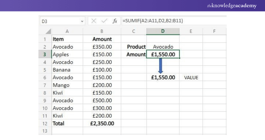
This example makes use of data on a list of fruits and their amount. The objective is to find the sum of a selected number of cells, holding the amount for Avocado. The result £1,550 is obtained upon using the Function:
=SUMIF(A2:A11,D2,B2:B11)
b) COUNTIF
The COUNTIF Function is also a widely used Function in Microsoft Excel. Identical to SUMIF, COUNTIF Function can only apply a single condition as well. At the need of applying multiple criteria, COUNTIFS Function can be used. The syntax for COUNTIF is:
=COUNTIF(range,criteria)
The following image is an example of using COUNTIF Function:
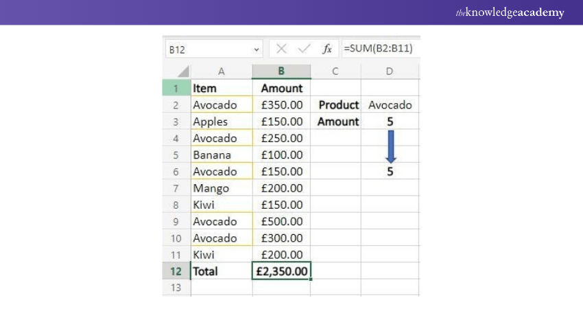
This image showcases the use of COUNTIF Function to count the number of times the word “Avocado” has been mentioned in the selected array of cells (A2:A11). The Function used to obtain the result of 5 is as follows:
=COUNTIF(A2:A11, "Avocado")
17) CONCATENATE

If you want to combine values from two or more cells into a single cell, you can use either the concatenate operator (&) or the CONCATENATE function in Excel.
The syntax for the CONCATENATE function is:
CONCATENATE(text1, [text2], ...)
For instance, to merge the values from cells A2 and B2, simply enter the following formula in another cell:
=CONCATENATE(A2, B2)
If you'd like to add a space between the combined values, you can include a space character (" ") within the arguments:
=CONCATENATE(A2, " ", B2)
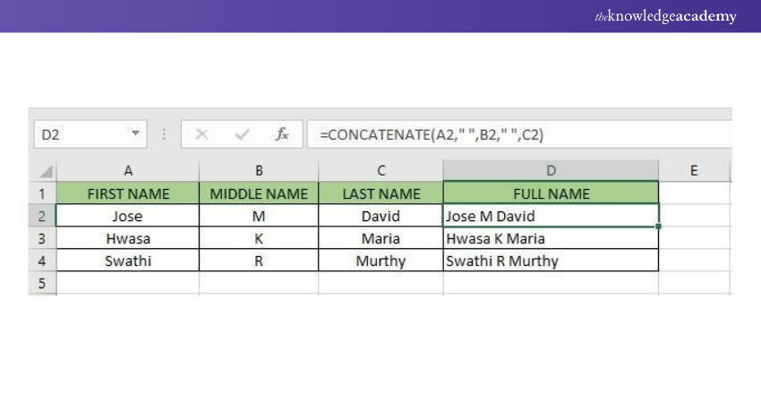
This allows you to easily join text, numbers, or both, into one cell using the CONCATENATE function in Excel.
18) CELL, LEFT, MID and RIGHT Functions
The CELL function in Excel can provide a range of information about the contents of a cell, including details like its column, row, location, and name. The syntax for using this function is:
=CELL(info_type, [reference])
The LEFT function is useful when you need to extract characters starting from the left side of a cell’s contents. It allows you to return a specified number of characters from the beginning of a text string. The LEFT function requires two arguments: the text you want to extract from and the number of characters to retrieve. The syntax is:
=LEFT(text, [num_chars])
Similarly, the MID function extracts text from the middle of a cell’s contents, starting from a specific position. It requires three arguments: the text string, the starting character position, and the number of characters to return. Its syntax is:
=MID(text, start_num, num_chars)
The RIGHT function works similarly to LEFT but extracts text from the right side of the cell. It uses two arguments: the selected text and the number of characters to extract from the end. The syntax is:
=RIGHT(text, [num_chars])
By combining these powerful Excel functions—CELL, LEFT, MID, and RIGHT—you can build advanced and complex formulas for more refined data manipulation.
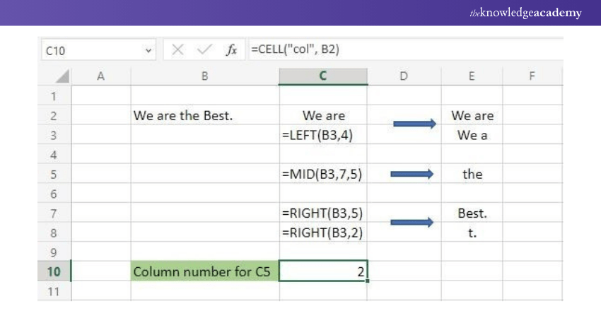
For example, you could use these functions to analyse a text string like "We are the Best" in various ways, as shown in the accompanying image.
19) XLOOKUP
XLOOKUP is an advanced function that is available only in Excel 2021 and Excel for Microsoft 365. The earlier versions of Excel will not be able to support this Microsoft Excel function. XLOOKUP is the latest and refined version of VLOOKUP. It addresses most of the drawback's VLOOKUP has. The syntax is as follows:
=XLOOKUP(lookup, lookup_array, return_array, [not_found], [match_mode], [search_mode])
The following image is an example of using the XLOOKUP Function in Excel:
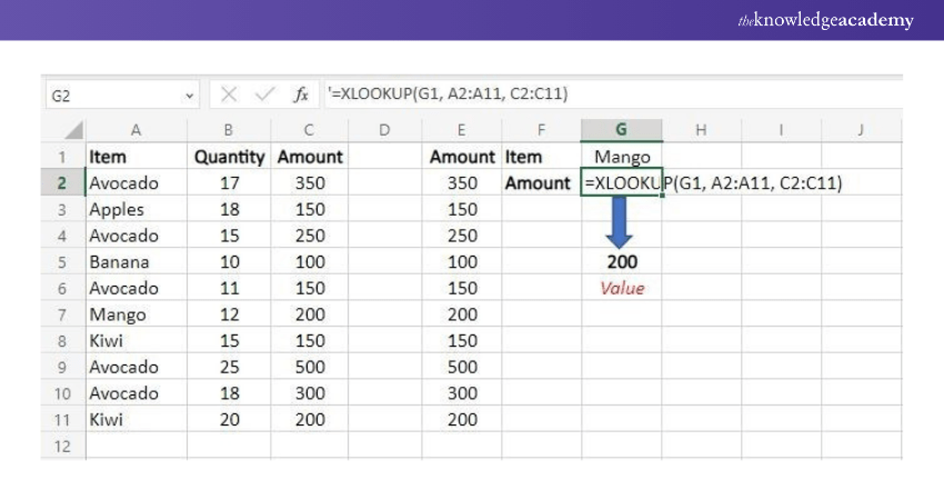
The above-mentioned example shows the use of multiple values to tally the result using XLOOKUP Function. Fruits, its quantity and amount are the factors being considered as data here. The Function used is as follows:
=XLOOKUP(G1, A2:A11, C2:C11)
20) VLOOKUP
To return a value in the same row from a specified column, the VLOOKUP Function does a vertical look up in the leftmost column. Let us translate this into everyday terms.
A serial number field in the home supply budget uniquely identifies each item in the budget. The VLOOKUP method can be used if you have the item serial number and want to get the item description. The syntax used is:
=VLOOKUP(lookup_value, table_array, column_index_num, [range_lookup])
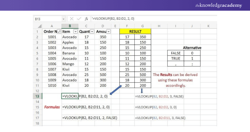
The above image uses an example based on order numbers, orders, their quantity and amount. The results obtained have used the Function in three different ways:
'=VLOOKUP(B2, B2:D2, 2, 0)
'=VLOOKUP(B2, B2:D11, 2, 0)
'=VLOOKUP(B2, B2:D11, 2, FALSE)
21) NOW()
The NOW() function in Excel returns both the current system date and time. It continuously updates based on your system's clock, so the result will always reflect the current date and time. This function is especially useful for tracking real-time changes in reports or time-sensitive calculations. The syntax is straightforward:
=NOW()
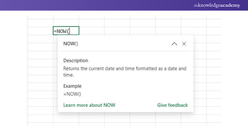
Keep in mind that since the NOW() function dynamically updates, any recalculation of your Excel sheet will change the output based on the latest system time.
22) TODAY()
The TODAY() function in Excel provides the current system date, without including the time. This function is ideal when you need the date for calculations or data that does not require time tracking. The result updates automatically as your system’s date changes. The syntax is:
=TODAY()
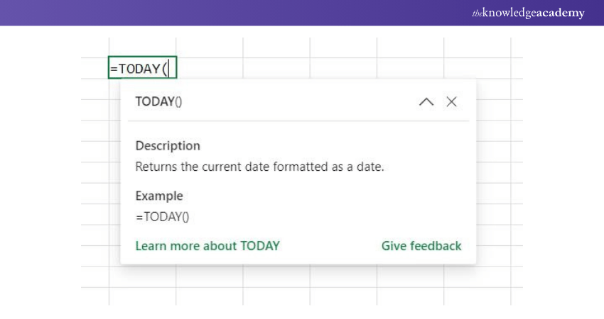
This simple function is useful for keeping track of dates in reports, logs, or time-sensitive analyses, with no need to manually update the date.
23) DATEDIF
The DATEDIF() function is one of the most commonly used formulas for working with time series data in Excel. It calculates the difference between two dates and returns the result in days, months, weeks, or years, depending on the unit specified.
For example, if you want to calculate the difference between two dates in days, you will specify "d" as the unit. It’s important to ensure that the first argument is the start date, and the second argument is the end date.
Here’s how it works in practice:
=DATEDIF(A2,B2,"d")
This formula will calculate the difference between the dates in cells A2 and B2 and return the result as the number of days. Always remember that the start date must be earlier than the end date for the formula to work correctly.
Learn Microsoft Excel more effectively with our Microsoft Excel Course. Sign up now!
Conclusion
Mastering Excel Formulas and Functions is essential for improving your data analysis and productivity. This blog has provided the key tools to help you work more efficiently and accurately. With these skills, you can now simplify complex tasks and enhance your reporting. Turn your passion for data into action and achieve more with confidence in Excel.
Want to learn how to create advanced formulas and macros in MS Excel? Sign up for our Microsoft Excel Expert Course now!
Frequently Asked Questions
What Excel Skills are Employers Looking for?

Employers typically seek skills such as Data Analysis, proficiency with formulas (SUM, IF, VLOOKUP), creating pivot tables, Data Visualisation through charts, familiarity with conditional formatting, and using advanced functions like INDEX-MATCH, macros, and automation with VBA.
What are the Best Practices for Writing Excel Formulas?

Ensure formulas are accurate by using cell references instead of hardcoding values. Keep formulas simple and readable by breaking down complex ones. Use parentheses to control calculation order, document formulas with comments, and test them with sample data to avoid errors.
What are the Other Resources and Offers Provided by The Knowledge Academy?

The Knowledge Academy takes global learning to new heights, offering over 3,000 online courses across 490+ locations in 190+ countries. This expansive reach ensures accessibility and convenience for learners worldwide.
Alongside our diverse Online Course Catalogue, encompassing 19 major categories, we go the extra mile by providing a plethora of free educational Online Resources like News updates, Blogs, videos, webinars, and interview questions. Tailoring learning experiences further, professionals can maximise value with customisable Course Bundles of TKA.
What is The Knowledge Pass, and How Does it Work?

The Knowledge Academy’s Knowledge Pass, a prepaid voucher, adds another layer of flexibility, allowing course bookings over a 12-month period. Join us on a journey where education knows no bounds.
What are the Related Courses and Blogs Provided by The Knowledge Academy?

The Knowledge Academy offers various Microsoft Excel Courses, including Microsoft Excel Course, Microsoft Excel VBA and Macro Training, and Excel for Accountants Course. These courses cater to different skill levels, providing comprehensive insights into Microsoft Excel.
Our Office Applications Blogs cover a range of topics related to PRINCE2, offering valuable resources, best practices, and industry insights. Whether you are a beginner or looking to advance your Project Management skills, The Knowledge Academy's diverse courses and informative blogs have you covered.
Upcoming Office Applications Resources Batches & Dates
Date
 Microsoft Excel Course
Mon 10th Mar 2025
Mon 7th Apr 2025
Mon 9th Jun 2025
Mon 8th Sep 2025
Mon 1st Dec 2025


 Top Rated Course


 If you wish to make any changes to your course, please


