We may not have the course you’re looking for. If you enquire or give us a call on 800969236 and speak to our training experts, we may still be able to help with your training requirements.
We ensure quality, budget-alignment, and timely delivery by our expert instructors.

MATLAB is a powerful programming language and an environment for numerical computation, visualisation, and algorithm development. It provides a flexible and interactive platform that allows users to perform various tasks, from simple calculations to complex data analysis, simulations, and modelling. In this blog, we will explore the power of MATLAB Commands for data analysis, simulations, modelling, image processing, & more. You can enhance your MATLAB skills with these essential Commands.
Table of Contents
1) Basic MATLAB Commands for working with the system and managing a session
2) MATLAB Commands for input and output
3) MATLAB Commands for vectors, matrices, and arrays
4) MATLAB Commands for plotting
5) MATLAB Commands for matrix
6) Conclusion
Basic MATLAB Commands for working with the system and managing a session
These basic general purposes of MATLAB Commands are invaluable for managing your MATLAB session. It also helps in accessing documentation, clearing the Command window, saving and loading variables, navigating directories, and interacting with the underlying Operating System.
When working with MATLAB, effectively managing your session can greatly enhance your workflow. Here are some essential commands for session management, including several commands that allow you to interact with the underlying operating system and perform system-related tasks. To further enhance your preparation, reviewing Matlab Interview Questions can help you better understand how these commands may be tested in interviews.
Understanding and utilising these Commands will help you streamline your workflow and improve your MATLAB skills.
|
Command |
Syntax |
Explanation |
|
help |
help functionName |
Displays information and documentation about a function |
|
clc |
clc |
Clears the Command window |
|
quit |
quit |
Terminates the MATLAB session |
|
save |
save fileName.mat variableName |
Saves variables or workspace to a file |
|
load |
load fileName.mat |
Loads variables or workspace from a file |
|
diary |
diary fileName.txt |
Logs all Commands and outputs to a text file |
|
cd |
cd folderPath |
Changes the current working directory |
|
dir |
dir |
Lists the contents of the current directory |
|
system |
system('Command') |
Executes a system Command from within MATLAB |
|
load |
load fileName.mat |
Loads previously saved variables and data from a file |
|
clear |
clear |
Removes all variables from the workspace |
|
clear var |
clear variableName |
Removes a specific variable from the workspace |
|
who |
who |
Lists all variables in the current workspace |
|
whos |
whos |
Provides detailed information about variables in the workspace |
|
workspace |
workspace |
Opens the workspace browser to view and modify variables |
|
isvarname |
isvarname('variableName') |
Checks if a string is a valid MATLAB variable name |
|
pwd |
pwd |
Returns the current working directory |
|
ls |
ls |
Lists files and directories in the current directory (UNIX-like) |
|
mkdir |
mkdir folderName |
Creates a new directory |
|
rmdir |
rmdir folderName |
Removes an empty directory |
|
delete |
delete fileName |
Deletes a file |
|
copyfile |
copyfile sourceFile destinationFolder |
Copies a file to a specified destination folder |
|
movefile |
movefile sourceFile destinationFolder |
Moves a file to a specified destination folder |
|
system |
system('Command') |
Executes a system Command from within MATLAB |
|
pause |
pause |
Pauses execution of a MATLAB program |
|
getenv |
getenv('variableName') |
Retrieves the value of an environment variable |
|
setenv |
setenv('variableName', 'value') |
Sets the value of an environment variable |
|
computer |
computer |
Returns the type of computer running MATLAB |
|
ispc |
ispc |
Checks if MATLAB is running on a Windows platform |
|
isunix |
isunix |
Checks if MATLAB is running on a UNIX-like platform |
|
ismac |
ismac |
Checks if MATLAB is running on a macOS platform |
Learn the essentials of MATLAB and SPSS with our MATLAB & SPSS Training and take your data analysis skills to the next level.
MATLAB Commands for input and output
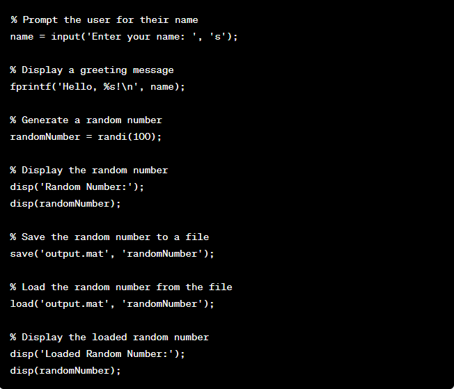
MATLAB provides several commands for handling input and output operations, allowing you to interact with users, read and write data, and perform file operations. Understanding Data Types in MATLAB is essential for working with these commands effectively. Here are some essential commands for input and output in MATLAB, including specialized functions such as MATLAB Convolution for advanced signal processing tasks.
1) input
variable = input('Prompt text: ');
Stores it in a variable by prompting the user for input.
2) disp
disp('Text to display');
Displays text or variables in the Command window.
3) fprintf
fprintf('Format string', variable1, variable2);
Writes formatted data to a file or the Command window.
4) fscanf
variable = fscanf(fileID, 'Format specifier');
Reads data from a file according to a specified format.
5) fprintf
fprintf(fileID, 'Format string', variable1, variable2);
Writes formatted data to a file.
6) fopen
fileID = fopen('fileName', 'mode');
Opens a file and returns a file identifier.
7) fclose
fclose(fileID);
Closes an open file.
8) fgetl
line = fgetl(fileID);
Reads a line of text from a file.
9) fgets
line = fgets(fileID);
Reads a line of text from a file, including newline characters.
9) fwrite
fwrite(fileID, data, 'precision');
Writes data to a file.
10) feof
feof(fileID)
Checks if the end of a file has been reached.
11) exist
exist('fileName', 'file')
Checks if a file or directory exists.
12) mkdir
mkdir('folderName')
Creates a new directory.
13) delete
delete('fileName')
Deletes a file or directory.

Learn how to use MATLAB Commands effectively with MATLAB Masterclass.
MATLAB Commands for vectors, matrices, and arrays
MATLAB is renowned for its powerful capabilities in handling vectors, matrices, and arrays. These Commands allow you to efficiently create, manipulate, and perform operations on multidimensional data structures. Here are some essential MATLAB Commands for working with vectors, matrices, and arrays.
These Commands enable you to create vectors, matrices, and matlab arrays of various sizes and initialise them with zeros, ones, random values, or identity matrices. You can also reshape, transpose, and tile matrices and calculate statistical properties such as minimum, maximum, sum, mean, and sort elements.
You can manipulate and perform operations on vectors, matrices, and arrays by leveraging these MATLAB Commands, enabling efficient data analysis, simulations, modelling, and more within your MATLAB workflow.
1) linspace
linspace(start, end, num)
Creates a row vector with equally spaced values between the start and endpoints. The 'num' parameter determines the number of values in the vector.
2) zeros
zeros(m, n)
Creates a matrix or array filled with zeros of size m-by-n. It is useful for initialising matrices before storing or manipulating data.
3) ones
ones(m, n)
Creates a matrix or array filled with ones of size m-by-n. It is commonly used for initialisation or generating matrices with specific dimensions.
4) eye
eye(n)
Creates an identity matrix of size n-by-n. The identity matrix has ones on the main diagonal and zeros elsewhere.
5) rand
rand(m, n)
Generates an m-by-n matrix or array filled with numbers ranging from 0 to 1 that are uniformly distributed. This Command is valuable for producing random data or initialising matrices with randomised values.
6) Size
size(matrix)
Returns the size of a matrix or array in the form of [rows, columns]. It provides information about the dimensions of the given matrix or array.
7) length
length(vector)
Returns the length of a vector, i.e., the number of elements in the vector. It is particularly useful for determining the size of a one-dimensional vector.
8) reshape
reshapedMatrix = reshape(originalMatrix, m, n)
Reshapes a matrix or array into a new size specified by m and n. It rearranges the elements of the original matrix to fit the desired dimensions.
9) transpose
transposedMatrix = originalMatrix
Transposes a matrix or array by interchanging its rows and columns. The transposed matrix is obtained by reflecting the original matrix along its main diagonal.
10) repmat
repeatedMatrix = repmat(originalMatrix, m, n)
Creates a tiled copy of a matrix or array, repeating it m times in the row direction and n times in the column direction. It is useful for replicating matrices or arrays to match desired dimensions.
11) min
minimumValue = min(vector)
Finds the minimum value in a vector. It returns the smallest element present in the given vector.
12) max
maximumValue = max(vector)
Finds the maximum value in a vector. It returns the largest element present in the given vector.
13) sum
sum(vector)
Calculates the sum of all elements in a vector. It returns the total sum of the values in the vector.
14) mean
mean(vector)
Calculates the mean (average) of the elements in a vector. It returns the arithmetic mean of the values in the vector.
15) sort
sortedVector = sort(vector)
Sorts the elements of a vector in ascending order. It rearranges the elements in the vector in a sorted manner.
16) isvector
isvector(matrix)
Checks if a matrix or array is a vector. It returns true if the given matrix or array has only one dimension, indicating it is a vector.
17) ismatrix
ismatrix(array)
Checks if an array is a matrix. It returns true if the given array has two dimensions, indicating it is a matrix.

MATLAB Commands for plotting
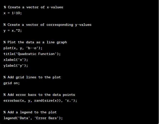
MATLAB projects offers a comprehensive set of plotting Commands that allow you to visualise and analyse data effectively. These Commands enable you to create various types of plots, customise their appearance, and add annotations. Here are some essential MATLAB plotting Commands.
1) plot
(plot(x, y))
Creates a 2D line plot using the values in vectors x and y. It is widely used to visualise the relationship between two variables or to represent data trends.
2) scatter
(scatter(x, y))
Creates a scatter plot using the values in vectors x and y. It is useful for visualising data point distribution and identifying patterns or clusters.
3) bar
(bar(x, y))
Creates a bar plot using the values in vectors x and y. It is commonly used to compare different categories or groups and display their corresponding values.
4) histogram
(histogram(data))
Creates a histogram plot to visualise the distribution of a dataset. It divides the data into bins and displays the frequency or count of values within each bin, a process often demonstrated using Histogram in MATLAB to effectively analyse and interpret data distributions.
5) pie
(pie(values, labels))
Creates a pie chart using the specified values and labels. It is useful for illustrating the proportions or percentages of different categories within a whole.
6) boxplot
(boxplot(data))
Creates a box plot to display the distribution of data. It shows the median, quartiles, and any outliers or extreme values concisely and visually informatively.
7) contour
(contour(X, Y, Z))
Creates a contour plot using the values in matrices X, Y, and Z. It represents 3D data on a 2D plane by displaying curves of constant values (contours) with varying heights.
8) surf
(surf(X, Y, Z))
Creates a surface plot using the values in matrices X, Y, and Z. It visualises 3D data as a surface with varying heights, allowing you to analyse complex relationships and patterns.
9) imagesc
(imagesc(data))
Creates a pseudocolour plot of a matrix or 2D array. It represents the values in the matrix using different colours, providing a visual representation of the data distribution.
10) quiver
(quiver(x, y, u, v))
Creates a 2D vector plot using the components of vectors u and v at the locations given by x and y. It is useful for visualising vector fields and directional information.
11) contourf
(contourf(X, Y, Z))
Creates a filled contour plot using the values in matrices X, Y, and Z. It is similar to the contour plot but fills the areas between contours with colours, enhancing the visual representation.
12) polarplot
(polarplot(theta, rho))
Creates a polar coordinate plot using the angles in theta and the distances from the origin in rho. It is suitable for visualising data with circular or angular relationships.
13) errorbar
(errorbar(x, y, y_err))
Creates an error bar plot using the values in vectors x, y, and y_err. It represents the uncertainty or error associated with each data point, providing a measure of variability.
14) stem
(stem(x, y))
Creates a stem plot to visualise discrete data. It displays vertical lines (stems) at the x-axis positions given by x with corresponding values y, making it useful for representing sequences or event data.

Step Up Your Coding Game! Explore MATLAB PDF Tutorials for Better Understanding.
MATLAB Commands for matrix
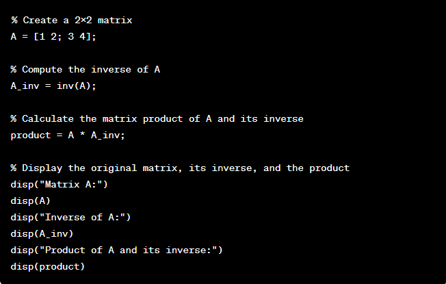
MATLAB, with its robust set of capabilities and supported by various MATLAB operators, offers a variety of matrix commands that streamline matrix manipulation, operations, and linear algebra calculations. These commands enable users to manipulate matrices, extract elements or submatrices, calculate matrix properties, and solve linear systems efficiently. However, it is important for users to be cautious of security concerns, such as shoulder surfing, especially when working with sensitive data or performing operations in public spaces. Here are some essential MATLAB matrix commands that contribute to the versatility of the software:
1) inv
inverseMatrix = inv(matrix)
Computes the inverse of a square matrix.
2) det
determinant = det(matrix)
Calculates the determinant of a square matrix.
3) rank
matrixRank = rank(matrix)
Determines the rank of a matrix.
4) eig
[eigenvalues, eigenvectors] = eig(matrix)
Computes the eigenvectors and eigenvalues of a square matrix.
5) trace
matrixTrace = trace(matrix)
Calculates the trace (sum of diagonal elements) of a matrix.
6) diag
diagonalMatrix = diag(vector)
Creates a diagonal matrix using the elements of a vector.
7) repmat
repeatedMatrix = repmat(matrix, m, n)
Creates a tiled copy of a matrix, repeating it m times in the row direction and n times in the column direction.
8) flipud
flippedMatrix = flipud(matrix)
Flips the matrix upside down (reverses the order of rows).
9) fliplr
FlippedMatrix fliplr(matrix)
Flips the matrix from left to right (reverses the order of columns).
10) transpose
transposedMatrix = matrix.
Transposes a matrix, interchanging its rows and columns.
11) repmat
repeatedMatrix = repmat(matrix, m, n)
Creates a tiled copy of a matrix, repeating it m times in the row direction and n times in the column direction.
12) reshape
reshapedMatrix = reshape(matrix, m, n)
Reshapes a matrix into a new size specified by m and n.
13) lu
[L, U, P] = lu(matrix)
Computes the LU factorisation of a matrix, where L is lower triangular, U is upper triangular, and P is the permutation matrix.
14) qr
[Q, R] = qr(matrix)
Computes the QR factorisation of a matrix, where Q is orthogonal, and R is upper triangular.
15) svd
[U, S, V] = svd(matrix)
Computes a matrix's singular value decomposition (SVD), S is a diagonal matrix, and U and V are orthogonal matrices.
16) chol
R = chol(matrix)
Computes the Cholesky factorisation of a positive definite matrix, where R is upper triangular.
17) pinv
pseudoInverseMatrix = pinv(matrix)
Computes the pseudo-inverse of a matrix using the Moore-Penrose inverse.
18) Norm
matrixNorm = norm(matrix)
Computes the norm (magnitude) of a matrix.
19) Solve
solutionVector = matrix rightHandSideVector or solutionVector = inv(matrix) * rightHandSideVector
It solves a linear system of equations using matrix inversion or the backslash operator.

Conclusion
Advantages of MATLAB Commands are a powerful toolset for beginners to explore the features of MATLAB in data analysis, simulations, modelling, and image processing. By learning and mastering these essential Commands, users can efficiently manage sessions, handle input and output devices, manipulate vectors, matrices, arrays, and more. With these Commands, users can streamline their data analysis workflow, gain insights from datasets, and customise visualisations to meet their specific needs.
Learn how to utilise the capabilities of SPSS with our SPSS Masterclass.
Upcoming Office Applications Resources Batches & Dates
Date
 MATLAB Course
Fri 13th Jun 2025
Fri 15th Aug 2025
Fri 10th Oct 2025
Fri 12th Dec 2025


 Top Rated Course


 If you wish to make any changes to your course, please


