


 Top Rated Course

We may not have the course you’re looking for. If you enquire or give us a call on + 1-866 272 8822 and speak to our training experts, we may still be able to help with your training requirements.
What is Time Complexity: Its Definition, Types, and Algorithms
Sienna Roberts 09 October 2023What is Time Complexity? Unravel the essence of time complexity and its role in algorithm analysis. Understand the significance it holds in evaluating the efficiency of algorithms. Learn the steps to calculate time complexity and explore the various types of time complexity. Delve into a comprehensive time complexity analysis of sorting algorithms, gaining insights into how they perform.

Training Outcomes Within Your Budget!
We ensure quality, budget-alignment, and timely delivery by our expert instructors.
Table of Contents

There is no ‘one-size-fits-all' solution to any problem in the computational world. There are various techniques, each with its own computational Time Complexity, power or other measurable metrics.
It is crucial to understand the mechanism of these techniques to select the optimal algorithm for solving a problem. Each algorithm is designed with a distinct operational order and Time Complexity, which influences the output of the algorithm’s execution. In this blog, you will learn that Time Complexity refers to the analysis of how an algorithm's runtime grows as the size of its input increases.
Table of Contents
1) What is Time Complexity?
2) Significance of Time Complexity
3) Steps to calculate the Time Complexity
4) Different types of Time Complexity
5) Time Complexity analysis of sorting algorithms
6) Time Complexity example
7) Conclusion
What is Time Complexity
Time Complexity is the amount of time that any algorithm takes to function. It is basically the function of the length of the input to the algorithm. Time Complexity measures the total time it takes for each statement of code in an algorithm to be executed.
Although it does not evaluate the execution time of the algorithm, it is intended to provide information associated with the increase or decrease in the execution time. This variation generally occurs with the increase or decrease in the number of operations in an algorithm.
Furthermore, just like any object is typically defined by time and space, an algorithm’s effectiveness can be determined by its Complexity in Space and Time. An algorithm is nothing but an instruction that tells a computer how it should execute a particular application program.
The algorithm’s execution time may differ for various inputs of equal size, and hence, the worst-case Time Complexity could be considered. This is the maximum time necessary for inputs of a fixed size.
For example, consider the problem of making tea. We can follow some key steps to prepare tea as shown below:
a) Step 1: Get a milk pan
b) Step 2: Gather milk, tea leaves, water and sugar.
I. Do we have milk?
A. If yes, add it to the mix of boiling water, tea leaves and sugar.
B. If not, do we need to purchase milk?
i. If yes, then go to the shop to buy.
ii. If no, terminate the process.
c) Step 3: Turn on the stove
The above steps are an example of a simple algorithm to make tea. In addition to following an algorithm, flowcharts can also be followed for executing a process.
Understand how algorithms work with data by signing up for our Data Structure and Algorithm Training now!
Significance of Time Complexity
Computer programming comprises algorithms, each of which is a finite sequence of well-defined instructions. These instructions are executed on a computer for Problem-solving and Decision-making. The computer always requires a fixed set of instructions, which can also contain variations for performing the same task, similar to the many possible ways to move a piece on a Rubik’s cube from one position to another.
Furthermore, developers also have a wide range of programming languages to choose from. Each programming language has a distinct structure for writing instructions, combined with the performance boundaries of the selected programming language. It is vital for developers to understand that the Types of Operating Systems, hardware, and processors in use have an influence on the execution of an algorithm.
Moreover, considering how various factors can significantly affect an algorithm’s outcome, developers should be careful to understand how computing systems perform a single task. They can determine this by assessing an algorithm’s space and Time Complexity.
On one hand, the space complexity of an algorithm helps determine the amount of memory or space it needs to operate as a function of its input length. On the other hand, the Time Complexity of the algorithm calculates the total time needed to complete the execution of a function on a specific length of input.
More importantly, an algorithm’s Time Complexity is significantly dependent on the size of the data being processed, and it also helps define the effectiveness of the algorithm. The algorithm’s Time Complexity is mainly an evaluation of its performance.
Steps to calculate the Time Complexity
Now, you have seen how each function is assigned an order notation and the relationship between the algorithm’s execution time, its number of operations and input data size.
The next step is to understand how you can evaluate an algorithm’s Time Complexity depending on its assigned order notation for each time it executes. The input size of the data to be processed and the run time of the computation for any given ‘n’ elements in the algorithm are also considered.
Here are the various steps that you can follow to evaluate the Time Complexity of an algorithm:
a) Step 1: The algorithm can be defined as a 2-input square matrix with the growth order ‘n’
b) Step 2: The np.random function is applied to select the values of every element in both matrices in a random manner
c) Step 3: A result matrix is then assigned to the algorithm, with 0 values of growth order equivalent to the order of the input matrix
d) Step 4: The resultant matrix is converted to a list-type
e) Step 5: Every element in the resultant list is then mathematically summed to derive a final answer
Pseudocode example
Here is an example of a pseudocode that helps demonstrate the concept of Time Complexity in algorithms. It analyses the algorithm with the Big O notation for growth order. This example demonstrates the operation of finding the maximum value in an array and calculating its Time Complexity:
function findMaxElement(arr):
if length(arr) == 0:
return "Array is empty"
max = arr[0] // Assume the first element is the maximum
for i from 1 to length(arr) - 1:
if arr[i] > max:
max = arr[i]
return max
The above pseudocode contains a data array ‘arr’, and here is how the Time Complexity is analysed to calculate the maximum value in it:
a) The if statement defined before the for loop evaluates if the array is devoid of elements. This operation is considered a constant time growth order, denoted as O (1).
b) The loop then proceeds to do iterations through all the elements in the array, starting from index[0] to [length(arr) - 1]. The worst-case scenario would be if the maximum value was at the last index or the end of the array or not present in the array. In this case, the above loop would run [length(arr) - 1] a number of times. Therefore, this demonstrates that there is a Time Complexity of the growth order O (n), where ‘n’ denotes the array’s length.
c) The variable assignment and the comparison formula in the loop are also called constant time operations, denoted as O (1).
The algorithm’s Time Complexity is always analysed by comparing the number of operations or iterations done in relation to the data input size.
Learn about data declarations and pointer techniques by signing up for C Programming now!
Different types of Time Complexity
Time Complexity is denoted by time as a function of the input’s length. A relationship also exists between the size of the input data, denoted as ‘n’, and the number of operations performed, denoted as ‘N’, in relation to time.
This relationship is commonly referred to as the ‘Order of Growth in Time Complexity’ and is denoted by ‘O[n],’ where ‘O’ symbolises the growth order and ‘n’ represents the input length. ‘O[n]’ is referred to as ‘Big O Notation’, which conveys an algorithm’s runtime and how quickly it grows with respect to the input ‘n.’
A prime example of an algorithm with Time Complexity O(n^2) is the ‘Selection sort’ algorithm. This algorithm is designed to perform an iteration through a list of numbers to ensure that the element at index ‘i’ is the ‘ith’ smallest/largest element in that list.
Furthermore, the Time Complexity notation comes in various forms, which are described as follows:
Constant Time Complexity: O (1)
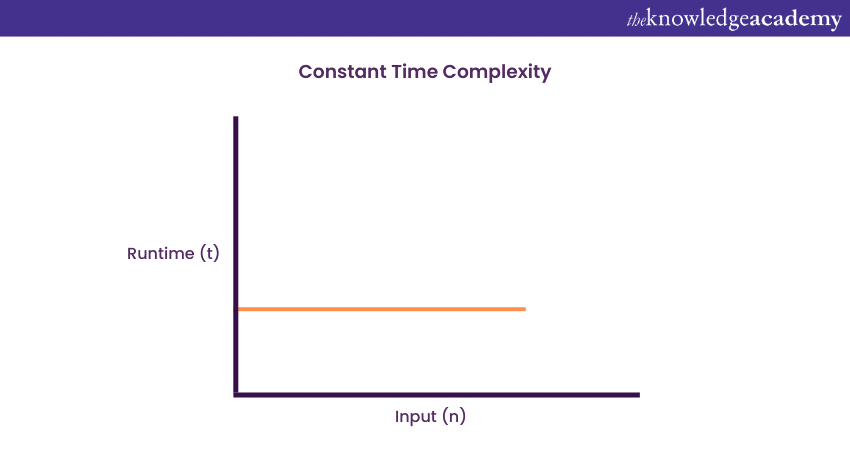
An algorithm will have a constant time with order O (1) if it is independent of the input size ‘n’. Regardless of what the input size ‘n’ is, the execution time will not be affected. The example of the Selection sort algorithm explained above demonstrates that no matter what the array (n) length may be, the final execution time to retrieve the first element in arrays of any length remains the same.
Now, the execution time can be considered as one unit of time, in which case it is only one unit of time’s worth to execute both arrays, regardless of their length. Therefore, the function will be considered under constant time with the growth order of O (1).
Linear Time Complexity: O (n)
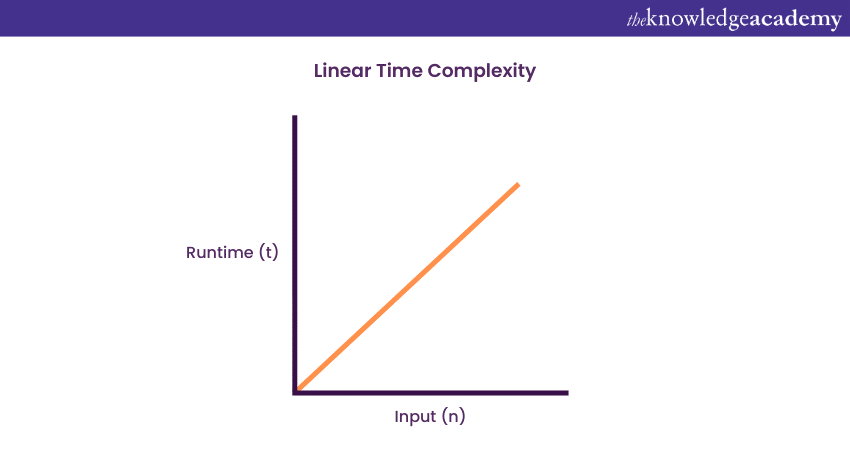
An algorithm will have a linear Time Complexity in the case when the execution time demonstrates a linear increase with the input’s length. The increase occurs when the function checks all the values in the processed input data, with the order O (n).
In the Selection sort algorithm, the execution time has a linear increase. Now, if the execution time is considered as one unit of time, then it will take [n*(1 unit time)] to execute the array to completion. Therefore, in growth order O (n), the function can be said to run linearly with the input size.
Logarithmic Time Complexity: O (log n)
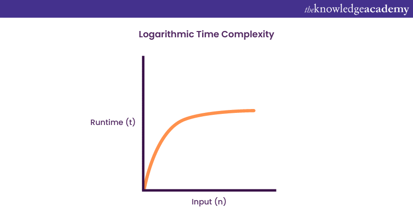
An algorithm will have a logarithmic Time Complexity in the case when the size of the input data is reduced in each step of the algorithm’s execution. The gradual reduction of the data size is an indication that the number of executions is not equal to the data input size; rather, they decrease with the increasing input size.
A good example of logarithmic Time Complexity is a binary search function, also known as a binary tree. Binary search functions involve the search of a given element in an array, followed by segregating the array into two sections. A new search is then performed in each section. The array split ensures that the operation is not performed on all elements in the data array.
Quadratic Time Complexity: O (n^2)
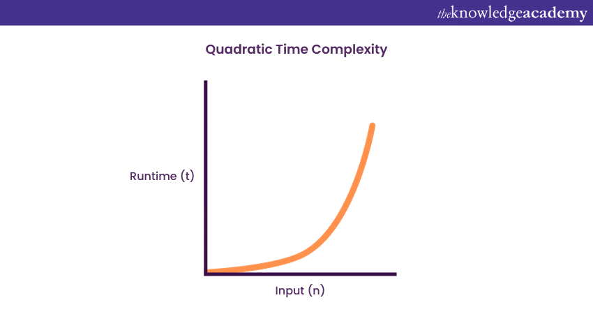
An algorithm will have a non-linear or quadratic Time Complexity in the case when the execution time increases in a non-linear fashion, I.e. (n^2) with the input data’s length. Nested loops are such algorithms that typically come under this growth order where one loop runs with the order O (n). If the algorithm involves a loop inside a loop, then it runs on the growth order of O (n)*O (n) = O (n^2).
Now, if there are ‘m’ number of loops defined in the structure of the function, the growth order is then denoted by O (n^m), which is basically called the ‘polynomial Time Complexity function’. The term means that an algorithm is called a solvable one in polynomial time if the number of steps needed to finish the algorithm for a given input is O (n^2) for a non-negative integer ‘t’, where n denotes the input data’s complexity.
Learn about object-oriented approaches, by signing up for our Object-Oriented Fundamentals Training now!
Time Complexity analysis of various sorting algorithms
The further exploration of the Time Complexity concept in different sorting algorithms helps you choose the optimal algorithm in any given situation. Sorting algorithms basically arrange an array’s elements in an ascending or descending order, resulting in a permutation of the input array. Here is a list describing the various sorting algorithms in detail:
Selection sort
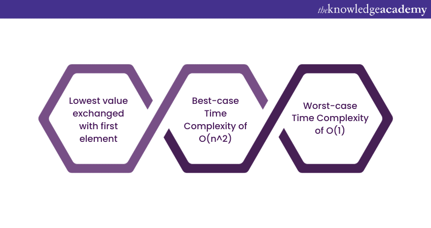
The Selection sort algorithm is a mathematical procedure where the lowest value is exchanged with the element in the first index position of the data array. This is followed by the second lowest value being exchanged with the element in the second index position of the array. This process is iterated over the remaining elements until all the elements of the array are sorted.
The Selection sort algorithm has a best-case Time Complexity of O (n^2) and a worst-case Time Complexity of O (1).
Merge sort
The Merge sort algorithm is an example of the ‘Divide and Conquer’ technique. The algorithm divides an array into equal halves and merges them back in a sorted order. The Merge sort is intended to continuously divide an array equally in recursions. Recursion is basically a technique for solving a computational problem, which entails the need to segregate the problem into smaller manageable parts to achieve the solution.
The Merge sort is basically a code written with a recursive function that calls itself within the same code, for solving the sorting problem. The Merge sort algorithm has a best-case Time Complexity of O (nlogn) and a worst-case Time Complexity of O (nlogn).
Bubble sort
The simplest of all sorting algorithms, the Bubble sort, is an algorithm that operates by iteratively swapping the values between two numbers. Also called the ‘Sinking sort’, the algorithm compares each element with the element in the index after it. The worst-case Time Complexity of the Bubble sort is O (n^2), and the best-case Time Complexity is O (n).
Quick sort
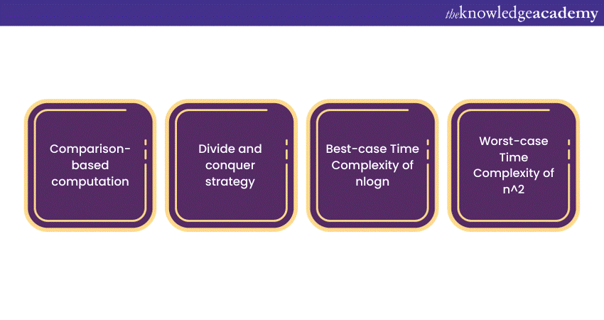
The Quick sort algorithm is the most well-known sorting algorithm for comparison-based computations. Similar to the Merge sort, this algorithm also functions on the Divide and conquer strategy.
It basically selects an array element as a pivot and partitions the array around the chosen element. The Quick sort algorithm is then applied recursively on the left partition, followed by the right partition. The best-case Time Complexity of the Quick sort is n*log (n), and the worst-case Time Complexity is n^2.
Heap sort
The Heap sort algorithm is among the various comparison-based sorting techniques. Its mechanism is similar to an optimised version of the Selection sort algorithm. It basically partitions the input array into sorted and unsorted sections, followed by iteratively shrinking the unsorted section. The shrink process occurs by removing the largest value from it and shifting it to the sorted section.
However similar it may be to the Selection sort, the Heap sort stands apart by not spending time scanning the unsorted section. More importantly, the Heap sort keeps the unsorted section in a heap data structure, which is a tree-based structure fulfilling the heap property. The best-case Time Complexity of the Quick sort is O (nlogn), and the worst-case Time Complexity is O (nlogn).
Bucket sort
The Bucket sort also called the ‘bin sort’ algorithm, is a sorting technique which distributes an array’s elements into multiple ‘buckets’. Each of these buckets is again sorted individually, either by applying another sorting technique or by recursively implementing the bucket sorting algorithm.
Each of the individual buckets is sorted with the Insertion sort algorithm before being joined together again. This sorting method has an exceptionally fast computational speed owing to the way the values are assigned to each bucket. The best-case Time Complexity for the Bucket sort technique is O (n + k), and the worst-case complexity is O (n ^ 2).
Insertion sort
The Insertion sort algorithm is a basic technique that sorts an array by computing one element with each iteration cycle. It takes an element and searches for its correct index in the sorted array. This sorting technique is quite akin to arranging a deck of playing cards.
The algorithm is deemed efficient owing to its organisational method on an unordered array of data through comparisons and element insertions based on either the numerical or alphabetical order. The best-case Time Complexity of the Insertion sort is (n), and the worst-case is (n^2).
Time Complexity example
Here is an example that will help you better understand the implementation of Time Complexity in a real-world scenario:
The ride-sharing application Uber, allows users to request a ride, followed by a search by the app to locate the nearest available driver to match their request. The search process by the application is then followed by sorting the located drivers to find the one in closest proximity to the user’s location.
Now, in this situation, there are two key approaches applied with respect to Time Complexity:
Linear search approach
Linear search is a fundamental approach implemented to locate an element in a dataset. It is designed to assess each element until a match is found. In the context of the application, the same approach is applied by iterating through a list of drivers available in the area, followed by a calculation of the distance between every driver’s and every user’s location.
The application then proceeds to select the driver in closest proximity to the user. It is also important to note that the application’s performance may degrade during peak hours.
Spatial indexing approach
The Spatial indexing approach is designed to locate elements in a specific region, calculate the closest neighbour or identify intersections between various spatial elements. This is an approach that computes data with more efficiency by utilising data structures such as Quadtrees or KD trees. These spatial indexing structures basically partition spaces into smaller regions, which enables quicker searches based on the spatial proximity of the element or object.
The Time Complexity of the Spatial indexing approach is close to O(log n), which is computationally more efficient than O(n). This approach is better because the search process is guided by the spatial indexing structure, which eliminates the comparison of distances between all located drivers.
Conclusion
We hope that you have understood the concept of Time Complexity and its significance while being applied in algorithms for searching and sorting arrays. It is vital to understand the Big ‘O’ notation associated with the best and worst-case time complexities of different algorithms to make the computation of arrays more efficient.
Learn the major programming languages by signing up for our Programming Training now!
Frequently Asked Questions
Upcoming Business Skills Resources Batches & Dates
Date
 Career Development Course
Career Development Course
Fri 17th Jan 2025
Career Development Course
Fri 21st Feb 2025
Career Development Course
Fri 4th Apr 2025
Career Development Course
Fri 6th Jun 2025
Career Development Course
Fri 25th Jul 2025
Career Development Course
Fri 7th Nov 2025
Career Development Course
Fri 26th Dec 2025
 If you wish to make any changes to your course, please


