We may not have the course you’re looking for. If you enquire or give us a call on 44 1344 203 999 and speak to our training experts, we may still be able to help with your training requirements.
Training Outcomes Within Your Budget!
We ensure quality, budget-alignment, and timely delivery by our expert instructors.
Deep Learning is a unique subset of Machine Learning that employs artificial neural networks, profound neural networks, to interpret and process data. So, if you are interested in learning in detail about Deep Learning, you need to understand What is Deep Learning Algorithm. The foundations of the Deep Learning Algorithm trace back to the structure of the human brain, which consists of interconnected layers of nodes or neurons.
According to Sttista, the global AI market will grow by over £1.20 trillion by 2030. The convergence of expansive datasets, advanced algorithms, and robust computing capabilities will make Deep Learning Algorithms hugely crucial in Artificial Intelligence and Machine Learning. In this blog, you will learn about What is Deep Learning Algorithm, the types of this Algorithm, and more. Read further to know more!
Table of Contents
1) What is Deep Learning Algorithm?
2) Types of Deep Learning Algorithms
a) Feedforward Neural Networks (FNN)
b) Convolutional Neural Networks (CNN)
c) Recurrent Neural Networks (RNN)
d) Long Short-Term Memory Networks (LSTMs)
e) Generative Adversarial Networks (GANs)
f) Autoencoders
g) Deep Belief Networks (DBN)
h) Radial Basis Function Neural Networks (RBFNN)
3) Conclusion
What is Deep Learning Algorithm?
Deep Learning, a unique subset of Machine Learning, has revolutionised numerous fields, from computer vision to natural language processing. It utilises artificial neural networks inspired by the human brain's interconnected neurons. These networks consist of several layers of neurons, allowing for the "depth" in Deep Learning. The depth enables these algorithms to process data in complex ways, extracting features and patterns that simpler algorithms might overlook.
A defining characteristic of Deep Learning is its ability to automatically learn such features from data, removing the need for manual feature extraction, which is often required in traditional Machine Learning. The algorithm refines its understanding as data progresses through a Deep Learning model's layer, gradually forming intricate and nuanced patterns. These algorithms don't operate in isolation. Their efficiency often hinges on vast datasets and powerful computational resources. Recent advances in Graphics Processing Unit (GPU) technology have significantly accelerated deep learning processes.
Types of Deep Learning Algorithms
There are numerous types of Deep Learning Algorithms. They are as follows:
Feedforward Neural Networks (FNN)
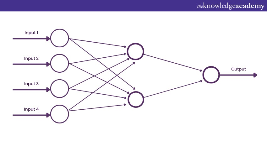
1) Basics: A basic neural network where information flows in one direction, from input to output. Think of them as the first bridge between traditional algorithms and the realm of neural networks. They connect input to output at their core, bypassing the need for recurrent loops.
a) Architecture: It comprises an input layer, one or more hidden layers, and an output layer. You can understand this from the following image:
b) Example use-case: Image classification, simple data regression.
2) Key points
a) Simplicity: Easiest to understand and implement.
b) Non-recurrence: No loops in the architecture, meaning it’s not recurrent.
3) Examples
a) Linear regression: The simplest form of FNN with no hidden layers.
b) Multi-Layer Perceptrons (MLP): FNNs with one or more hidden layers.
4) Advanced features
a) Activation functions: Determines the output of a neuron. Standard procedures include sigmoid, tanh, and ReLU.
b) Loss functions: It measures the difference between actual and predicted output. Examples include Mean Squared Error for regression tasks and Cross-Entropy for classification.
5) Advanced example use-cases
a) Credit scoring: FNN can be utilised to determine the creditworthiness of an individual based on historical data.
Every Learning Algorithm has a way of measuring mistakes, and for FNNs, this measure comes from loss functions. Mean Squared Error (MSE) and Cross-Entropy Loss are the most widely used. While MSE measures the average squared difference between actual and predicted values, Cross-Entropy measures the dissimilarity between actual and predicted probabilities.
One intriguing use of FNNs lies in credit scoring. By inputting historical financial data, banks can harness FNNs to gauge the likelihood of an individual defaulting on a loan. This automated risk assessment has transformed the finance sector, making credit decisions swifter and often more objective.
Enhance your knowledge of Deep Learning with our Deep Learning Training! Join now!
Convolutional Neural Networks (CNN)
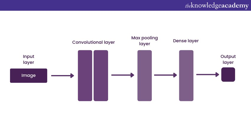
1) Basics: CNN is another Deep Learning Algorithm primarily used for image recognition. Unlike other networks, CNNs can automatically and adaptively learn spatial hierarchies of features from images. This makes them invaluable for tasks ranging from facial recognition in security systems to medical diagnoses from X-rays.
a) Architecture: Includes convolutional layers that apply filters to input, pooling layers, and fully connected layers. You can understand this better from this image:
b) Example use-case: Object detection, facial recognition.
2) Key points
a) Feature learning: Automatically learns features from images.
b) Translation invariance: Can recognise objects irrespective of their position in the image.
3) Examples
a) LeNet: One of the earliest CNNs used for digit recognition.
b) VGGNet: Known for its simplicity and effectiveness in image recognition.
4) Advanced features
a) Pooling layers: Reduces the spatial size, making the network faster and less prone to overfitting. Max pooling and average pooling are commonly used.
b) Dropout: A regularisation technique to prevent overfitting. Randomly selected neurons are ignored during training.
5) Advanced example use-case
a) Medical imaging: CNNs help in detecting anomalies in X-rays or MRI scans.
CNN’s convolution operation filters input data to extract high-level features. Pooling layers then condense this data, reducing computational demands and mitigating the risk of overfitting. Together, they distil images into their most salient and informative features.
The process from the input image to classification involves transforming pixels into patterns. For instance, in diagnosing diseases from medical scans, CNNs might identify edges, shapes, and specific anatomical markers indicative of disease.
Are you interested in learning Machine Learning and Artificial Intelligence? Register for our Artificial Intelligence & Machine Learning Training!
Recurrent Neural Networks (RNN)
1) Basics: It is effective for sequential data like time series or language. While FNNs and CNNs perceive inputs as isolated units, RNNs recognise the importance of sequences. They are designed to remember previous inputs using their internal memory. This makes them perfect for time series predictions like stock market forecasting or natural language processing tasks.
a) Architecture: Includes loops to allow information persistence.
b) Example use-case: Natural language processing, stock market prediction.
2) Key points
a) Sequential processing: Can process sequences of data.
b) Long-range dependencies: Struggles with learning long-range temporal dependencies.
3) Examples
a) Elman networks: Simple RNNs for tasks like sequence prediction.
b) Jordan networks: Variants of RNNs with backward connections.
4) Advanced features
a) Vanishing gradient problem: RNNs can suffer from gradients that either vanish or explode, making training difficult. This is addressed in LSTMs and GRUs.
b) Gated Recurrent Units (GRUs): A variation of RNNs that tackles the vanishing gradient problem.
5) Advanced example use-case
a) Sentiment analysis: RNNs analyse the sentiment of textual data like movie reviews.
However, traditional RNNs come with pitfalls. They struggle with long-term dependencies due to the vanishing (or occasionally, exploding) gradient problem. This is where the gradients used to update network weights become too small for effective learning or too large, causing overshooting.
RNNs have found their stride in applications that involve sequences, particularly language. Sentiment analysis, for instance, leverages RNNs to gauge public sentiment, parsing sentences to deduce whether a product review is positive or negative.
Empower your tech journey with our Machine Learning Training. Sign up now!
Long Short-Term Memory Networks (LSTMs)
1) Basics: It is a special kind of RNN and Deep Learning Algorithms which is effective for long-range dependencies. LSTMs, a particular type of RNN, were introduced to overcome the limitations of traditional RNNs. They excel at remembering information for extended periods, making them exceptional for tasks like speech recognition.
a) Architecture: Similar to RNN but with a complex cell structure in hidden layers.
b) Example use-case: Speech recognition, machine translation.
2) Key points
a) Long-range dependencies: Excels at learning from long sequences.
b) Versatility: Widely used in various time-series applications.
3) Examples
a) Seq2Seq models: LSTMs for tasks like machine translation.
b) Music generation: LSTMs can generate melodies based on prior musical sequences.
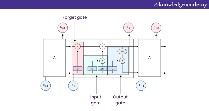
4) Advanced features: LSTMs introduce concepts of gates: forget, input, and output gates. These gates determine how much information should be stored, discarded, or passed to the next layer, giving LSTMs unparalleled memory capabilities.
a) Forget gate: This decides what information should be discarded from the cell state.
b) Input and output gates: Controls the updating and outputting of the cell state.
5) Advanced example use-case
a) Predictive text input: LSTMs can predict the next word in a sequence, aiding in faster typing.
LSTMs shine brightly in applications like machine translation. Platforms like Google Translate rely heavily on them to convert one language to another, harnessing their ability to understand context and nuance in sequences of words. The below image will clarify this further:
Generative Adversarial Networks (GANs)
1) Basics: GANs are innovative Deep Learning models that generate new data resembling a given set. It creates an artwork and also determines its authenticity. It comprises two networks - the generator generates data, and the discriminator evaluates it. The following image will help you to understand better:
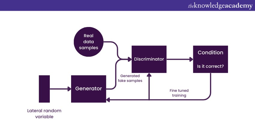
a) Architecture: Uses both a generative and a discriminative model.
b) Example use-case: Art creation, data augmentation.
2) Key points
a) Adversarial training: Trains in a contest, improving both generator and discriminator.
b) Creative outputs: Known for generating new, realistic data.
3) Examples
a) StyleGAN: Generates realistic human faces.
b) CycleGAN: Transfers styles between unrelated image domains.
4) Advanced features
a) Latent space: GANs generate data from random points in this latent space.
b) Mode collapse: A situation where the generator yields limited samples.
5) Advanced example use-case
a) Super-resolution: GANs can enhance the resolution of images, making them more explicit.
This continuous game between the Generator and Discriminator ensures that the generated data is increasingly refined and realistic. Over time, the Generator becomes so adept that the Discriminator can hardly tell what is real from what is fake.
GANs are making waves in creative domains. Whether generating art pieces that auction for exorbitant sums or creating lifelike video game environments, GANs redefine the boundaries of machine creativity.
Deepen your AI expertise with our Deep Learning with TensorFlow Training
Autoencoders
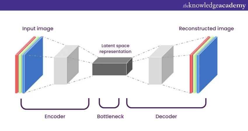
1) Basics: Autoencoders are one of the Deep Learning Algorithms which are unsupervised neural networks that aim to copy their inputs to their outputs. They compress the input into a dense representation and then reconstruct it. They're like learning an efficient data codec from scratch. They are used for unsupervised learning tasks like data compression.
a) Architecture: Consists of an encoder that compresses input and a decoder that reconstructs it.
b) Example use-case: Anomaly detection, feature learning.
2) Key points
a) Data-specific: Tailored to specific kinds of data.
b) Dimensionality reduction: Effective for reducing the number of variables in data.
3) Examples
a) Sparse autoencoder: Used in feature learning.
b) Denoising autoencoder: Used to remove noise from images.
4) Advanced features
a) Variational Autoencoders (VAEs): An autoencoder that adds probabilistic encoders and decoders.
b) Contractive autoencoder: Focuses on learning a robust representation of slight variations of the input data.
5) Advanced example use-case
a) Image colourisation: Transforming black and white images into colour.
While they're excellent for data compression, autoencoders' ability to reduce dimensionality has other merits. They're pivotal in anomaly detection. By learning to recreate 'normal' data, autoencoders can flag data that deviates from the norm, making them invaluable in cybersecurity.
One fascinating application of autoencoders is image colourisation. Given a black-and-white image, autoencoders can predict and apply colour, turning grayscale photographs into vibrant-coloured versions.
Improve your Artificial Intelligence skills – Register now in our Artificial Intelligence (AI) For Project Managers
Deep Belief Networks (DBN)
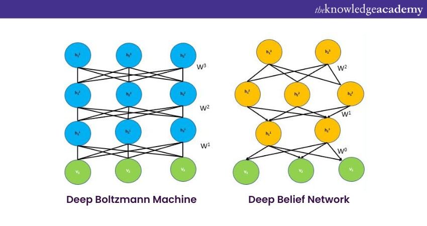
1) Basics: DBNs are architectures comprising multiple layers of stochastic, latent variables. They're a stack of Restricted Boltzmann Machines (RBMs) where the output of each layer serves as input for the next.
a) Architecture: Includes multiple layers of stochastic, latent variables.
b) Example use-case: Dimensionality reduction, classification.
2) Key points
a) Unsupervised pre-training: Can be pre-trained layer by layer.
b) Fine-tuning: Usually followed by backpropagation for fine-tuning.
3) Examples
a) Image recognition: Used in early layers to recognise basic shapes.
b) Document retrieval: Effective for searching through a large set of documents.
4) Advanced features
a) Energy-based models: DBNs are energy-based, meaning they associate scalar energy with every configuration of the variables in the network.
b) Contrastive divergence: A popular method for training RBMs, which form the layers of a DBN.
5) Advanced example use-case
a) Audio recognition: DBNs can be used to detect and classify sound patterns.
DBNs adopt a unique two-step training process. The first involves greedily training each RBM layer-by-layer, followed by a fine-tuning phase using traditional backpropagation. These also find extensive applications in areas demanding high-level feature extraction. Whether it's distinguishing different genres of music based on their audio signatures or analysing deep-space telescope data to pinpoint distant galaxies, DBNs distil data into actionable insights.
Do you want to learn the importance of neural networks? Sign up for our Neural Networks with Deep Learning Training
Radial Basis Function Neural Networks (RBFNN)
1) Basics: Radial Basis Function Neural Networks, often abbreviated as RBFNN, are a distinctive type of neural network known for their unique activation function. Unlike traditional Feedforward Neural Networks that utilise sigmoidal or ReLU-based activation functions, RBFNNs employ radial basis functions as their activation function.
This uniqueness allows them to approximate any continuous function accurately, provided they have a sufficient number of hidden neurons. Emphasises the distance between data points and a fixed centre.
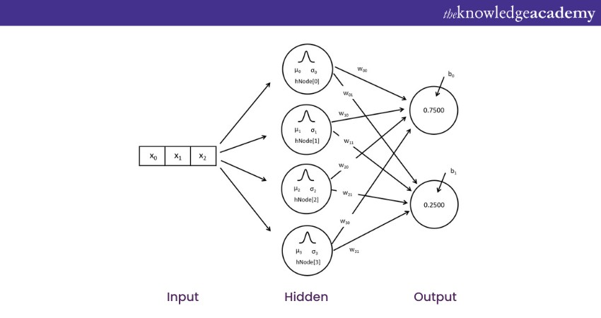
a) Architecture: Similar to FNN but uses radial basis functions as activation functions. RBFNN also primarily consist of three layers:
1) Input layer: It receives the raw input data like any other neural network.
2) Hidden layer: This is where the magic of RBFs happens. Each neuron in this layer contains a centre associated with it. When an input is provided, the neuron calculates the distance between the input and its centre and then applies the RBF.
3) Output layer: Based on the activations from the hidden layer, this layer produces the final prediction or classification.
4) Example use-case: Pattern recognition, function approximation.
2) Key points
a) Non-linear mapping: Maps input to a higher-dimensional space.
b) Interpolation: Well-suited for tasks that require interpolation between data points.
3) Examples
a) Time series prediction: RBFNNs can be used to predict future values in a sequence.
b) Medical diagnosis: Used to make predictions or decisions without human intervention.
4) Advanced features
a) Centres: Every neuron in the hidden layer of an RBFNN is a centre. The closer the input feature vector is to the centre of a neuron, the larger the neuron's output.
b) Spread (or radius): Determines the region of influence of a neuron.
5) Advanced example use-case
a) Robot control: RBFNNs can control robot movements in dynamic environments.
RBFNNs are one of the Deep Learning Algorithms which excel in areas where the relationship between inputs and outputs is intricate and non-linear. Their ability to provide localised sensitivity to particular regions of the input space makes them ideal for tasks like function approximation, time series prediction, and even robot control systems.
This is where precision and sensitivity to specific input patterns are crucial. RBFNNs can be computationally expensive, especially when determining centres for large datasets. Moreover, the choice of the spread and the number of centres can significantly influence the network's performance, requiring meticulous tuning.
Variational Autoencoders (VAEs)
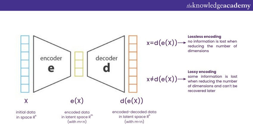
Variational Autoencoders, often abbreviated as VAEs, are a specialised type of autoencoder designed for generative tasks. They merge the principles of Deep Learning with probabilistic graphical modelling to produce new instances that can closely resemble the input data. Unlike traditional autoencoders, which aim to encode an input and then decode it back to the original with minimal loss, VAEs are one of a king Deep Learning Algorithm which introduces a probabilistic twist.
Instead of encoding an input to a fixed "code" in the latent space, VAEs encode input data into a distribution (usually Gaussian). During decoding, a point from this distribution is sampled to reconstruct the input. This stochastic process ensures the generated data has variations, making VAEs excellent for generative tasks.
1) Applications:
VAEs find widespread use in various domains, notably:
a) Where image generation is new and unseen images need to be generated.
b) Denoising, where VAEs can recover clean photos from noisy counterparts.
c) Anomaly detection since VAEs trained on standard data will have difficulty reconstructing anomalies.
2) Key advantage:
The beauty of VAEs lies in their ability to manage and introduce controlled randomness, ensuring the generation of diverse yet coherent outputs. Their probabilistic nature also offers robustness and versatility compared to deterministic models like standard autoencoders.
Self-Organising Maps (SOMs)
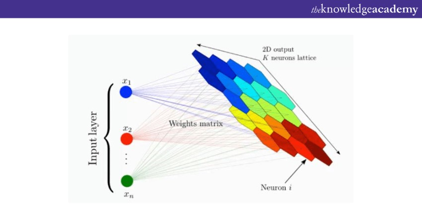
Self-Organising Maps, or SOMs, are a type of unsupervised neural network model. They are particularly adept at visualising high-dimensional data in a lower-dimensional space (typically 2D). SOMs work by iteratively adjusting neuron weights to resemble clusters of the input data. Each neuron in the network represents a position in this low-dimensional output space.
The neuron with weights most similar to that input (often termed the "winning neuron") is identified when presented with an input. This winning neuron and its neighbours are adjusted closer to that input. Over time, the map self-organises to produce a representation that captures the inherent topologies and relationships of the input data.
1) Applications:
SOMs have a plethora of uses:
a) Data visualisation offers insights into the underlying structure of data.
b) Clustering, where data points that fall under the same neuron or neighbouring neurons can be considered a cluster.
c) Anomaly detection, as outliers may not be well-represented by any neuron.
2) Key advantage:
The unique capability of SOMs to preserve the topological properties of the input space in the reduced output space sets them apart. This results in a meaningful visualisation where data points close in the input space remain close in the 2D representation.
Conclusion
We hope that you understood What is Deep Learning Algorithm from this blog. In this blog, we discussed how it harnesses neural networks to mimic human-like data processing for complex tasks. This comprehensive overview highlighted their versatility, from VAEs for generative studies to Self-Organising Maps (SOMs). As technology evolves, these algorithms will be pivotal in advancing AI solutions.
Combine Excel with Machine Learning – Sign up now for our AI And ML With Excel Training.
Frequently Asked Questions
Upcoming Data, Analytics & AI Resources Batches & Dates
Date
 Deep Learning Course
Fri 17th Jan 2025
Fri 7th Mar 2025
Fri 23rd May 2025
Fri 18th Jul 2025
Fri 12th Sep 2025
Fri 12th Dec 2025


 Top Rated Course


 If you wish to make any changes to your course, please


